
Example 3 - stripy interpolation on the sphere
Contents
Example 3 - stripy interpolation on the sphere
SSRFPACK is a Fortran 77 software package that constructs a smooth interpolatory or approximating surface to data values associated with arbitrarily distributed points on the surface of a sphere. It employs automatically selected tension factors to preserve shape properties of the data and avoid overshoot and undershoot associated with steep gradients.
The next three examples demonstrate the interface to SSRFPACK provided through stripy
Notebook contents
The next example is Ex4-Gradients
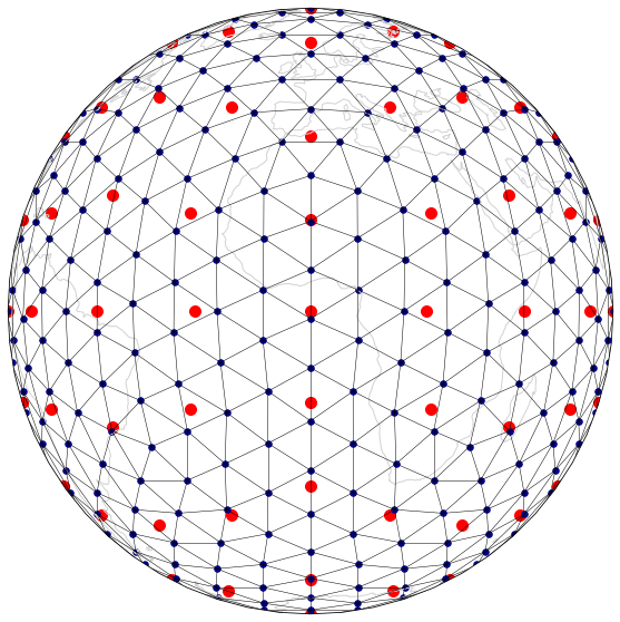
Define two different meshes
Create a fine and a coarse mesh without common points
import stripy as stripy

cmesh = stripy.spherical_meshes.triangulated_cube_mesh(refinement_levels=2)
fmesh = stripy.spherical_meshes.icosahedral_mesh(refinement_levels=2, include_face_points=True)

print(cmesh.npoints)
print(fmesh.npoints)
98
482
help(cmesh.interpolate)
Help on method interpolate in module stripy.spherical:

interpolate(lons, lats, zdata, order=1, grad=None, sigma=None) method of stripy.spherical_meshes.triangulated_cube_mesh instance
    Base class to handle nearest neighbour, linear, and cubic interpolation.
    Given a triangulation of a set of nodes on the unit sphere, along with data
    values at the nodes, this method interpolates (or extrapolates) the value
    at a given longitude and latitude.

    Args:
        lons : float / array of floats, shape (l,)
            longitudinal coordinate(s) on the sphere
        lats : float / array of floats, shape (l,)
            latitudinal coordinate(s) on the sphere
        zdata : array of floats, shape (n,)
            value at each point in the triangulation
            must be the same size of the mesh
        order : int (default=1)
            order of the interpolatory function used

            - `order=0` = nearest-neighbour
            - `order=1` = linear
            - `order=3` = cubic

        sigma : array of floats, shape (6n-12)
            precomputed array of spline tension factors from
            `get_spline_tension_factors(zdata, tol=1e-3, grad=None)`
            (only used in cubic interpolation)

    Returns:
        zi : float / array of floats, shape (l,)
            interpolated value(s) at (lons, lats)
        err : int / array of ints, shape (l,)
            whether interpolation (0), extrapolation (1) or error (other)
%matplotlib inline

import cartopy
import cartopy.crs as ccrs
import matplotlib.pyplot as plt
import numpy as np


def mesh_fig(mesh, meshR, name):

    fig = plt.figure(figsize=(10, 10), facecolor="none")
    ax  = plt.subplot(111, projection=ccrs.Orthographic(central_longitude=0.0, central_latitude=0.0, globe=None))
    ax.coastlines(color="lightgrey")
    ax.set_global()

    generator = mesh
    refined   = meshR

    lons0 = np.degrees(generator.lons)
    lats0 = np.degrees(generator.lats)

    lonsR = np.degrees(refined.lons)
    latsR = np.degrees(refined.lats)

    lst = generator.lst
    lptr = generator.lptr


    ax.scatter(lons0, lats0, color="Red",
                marker="o", s=100.0, transform=ccrs.PlateCarree())

    ax.scatter(lonsR, latsR, color="DarkBlue",
                marker="o", s=30.0, transform=ccrs.PlateCarree())

    segs = refined.identify_segments()

    for s1, s2 in segs:
        ax.plot( [lonsR[s1], lonsR[s2]],
                 [latsR[s1], latsR[s2]],
                 linewidth=0.5, color="black", transform=ccrs.Geodetic())

    # fig.savefig(name, dpi=250, transparent=True)

    return

mesh_fig(cmesh,  fmesh, "Two grids" )
Analytic function
Define a relatively smooth function that we can interpolate from the coarse mesh to the fine mesh and analyse
def analytic(lons, lats, k1, k2):
     return np.cos(k1*lons) * np.sin(k2*lats)

coarse_afn = analytic(cmesh.lons, cmesh.lats, 5.0, 2.0)
fine_afn   = analytic(fmesh.lons, fmesh.lats, 5.0, 2.0)
The analytic function on the different samplings
It is helpful to be able to view a mesh in 3D to verify that it is an appropriate choice. Here, for example, is the icosahedron with additional points in the centroid of the faces.
This produces triangles with a narrow area distribution. In three dimensions it is easy to see the origin of the size variations.
import k3d
plot = k3d.plot(camera_auto_fit=False, grid_visible=False,
                menu_visibility=False, axes_helper=False )

findices = fmesh.simplices.astype(np.uint32)
cindices = cmesh.simplices.astype(np.uint32)
fpoints = np.column_stack(fmesh.points.T).astype(np.float32)
cpoints = np.column_stack(cmesh.points.T).astype(np.float32)

plot   += k3d.mesh(fpoints, findices, wireframe=False, color=0xBBBBBB,
                   flat_shading=True, opacity=1.0 )


plot   += k3d.points(fpoints, point_size=0.01,color=0xFF0000)


plot   += k3d.points(cpoints, point_size=0.02,color=0x00FF00)

plot.display()
Interpolation from coarse to fine
The interpolate method of the sTriangulation takes arrays of longitude, latitude points (in radians) and an array of
data on the mesh vertices. It returns an array of interpolated values and a status array that states whether each value
represents an interpolation, extrapolation or neither (an error condition). The interpolation can be nearest-neighbour (order=0),
linear (order=1) or cubic spline (order=3).
interp_c2f1, err = cmesh.interpolate(fmesh.lons, fmesh.lats, order=1, zdata=coarse_afn)
interp_c2f3, err = cmesh.interpolate(fmesh.lons, fmesh.lats, order=3, zdata=coarse_afn)

err_c2f1 = interp_c2f1-fine_afn
err_c2f3 = interp_c2f3-fine_afn
interp_c2f1.max()
0.9118629302784801
import k3d
plot = k3d.plot(camera_auto_fit=False, grid_visible=False,
                menu_visibility=True, axes_helper=False )

findices = fmesh.simplices.astype(np.uint32)
cindices = cmesh.simplices.astype(np.uint32)
fpoints = np.column_stack(fmesh.points.T).astype(np.float32)
cpoints = np.column_stack(cmesh.points.T).astype(np.float32)


plot   += k3d.mesh(fpoints, findices, wireframe=False, attribute=interp_c2f1,
                   color_map=k3d.colormaps.basic_color_maps.CoolWarm,
                   name="1st order interpolant",
                   flat_shading=False, opacity=1.0  )


plot   += k3d.mesh(fpoints, findices, wireframe=False, attribute=interp_c2f3,
                   color_map=k3d.colormaps.basic_color_maps.CoolWarm,
                   name="3rd order interpolant",
                   flat_shading=False, opacity=1.0  )


plot   += k3d.mesh(fpoints, findices, wireframe=False, attribute=err_c2f1,
                   color_map=k3d.colormaps.basic_color_maps.CoolWarm,
                   name="1st order error",
                   flat_shading=False, opacity=1.0  )


plot   += k3d.mesh(fpoints, findices, wireframe=False, attribute=err_c2f3,
                   color_map=k3d.colormaps.basic_color_maps.CoolWarm,
                   name="3rd order error",
                   flat_shading=False, opacity=1.0  )


plot   += k3d.points(fpoints, point_size=0.01,color=0x779977)


plot.display()
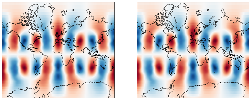
Interpolate to grid
Interpolating to a grid is useful for exporting maps of a region. The interpolate_to_grid method interpolates mesh data to a regular grid defined by the user. Values outside the convex hull are extrapolated.
interpolate_to_gridis a convenience function that yields identical results to interpolating over a meshed grid using theinterpolatemethod.
resX = 200
resY = 100

extent_globe = np.radians([-180,180,-90,90])

grid_lon = np.linspace(extent_globe[0], extent_globe[1], resX)
grid_lat = np.linspace(extent_globe[2], extent_globe[3], resY)

grid_z1 = fmesh.interpolate_to_grid(grid_lon, grid_lat, interp_c2f3)

# compare with `interpolate` method
grid_loncoords, grid_latcoords = np.meshgrid(grid_lon, grid_lat)

grid_z2, ierr = fmesh.interpolate(grid_loncoords.ravel(), grid_latcoords.ravel(), interp_c2f3, order=3)
grid_z2 = grid_z2.reshape(resY,resX)
fig = plt.figure(figsize=(15, 10), facecolor="none")

ax1  = plt.subplot(121, projection=ccrs.Mercator())
ax1.coastlines()
ax1.set_global()
ax1.imshow(grid_z1, extent=np.degrees(extent_globe), cmap='RdBu', transform=ccrs.PlateCarree())

ax2  = plt.subplot(122, projection=ccrs.Mercator())
ax2.coastlines()
ax2.set_global()
ax2.imshow(grid_z2, extent=np.degrees(extent_globe), cmap='RdBu', transform=ccrs.PlateCarree())
<matplotlib.image.AxesImage at 0x14fb1ce80>
The next example is Ex4-Gradients