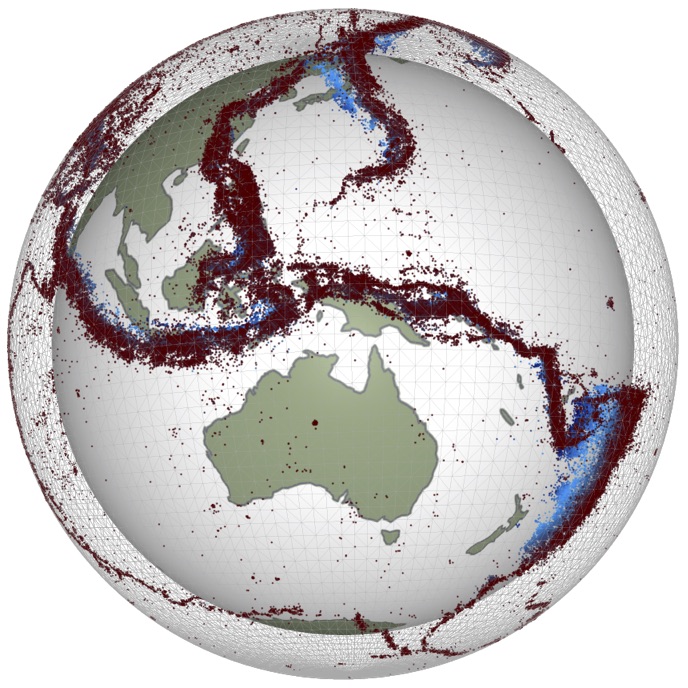
Example 1 - Triangulation of arbitrary points on the sphere
Contents
Example 1 - Triangulation of arbitrary points on the sphere
stripy provides a python interfact to STRIPACK and SSRFPACK (Renka 1997a,b) as a triangulation class that would typically be used as follows:
import stripy as stripy
spherical_triangulation = stripy.sTriangulation(lons=vertices_lon_as_radians, lats=vertices_lat_as_radians)
s_areas = spherical_triangulation.areas()
The methods of the sTriangulation class include interpolation, smoothing and gradients (from SSRFPACK), triangle areas, point location by simplex and nearest vertex, refinement operations by edge or centroid, and neighbourhood search / distance computations through a k-d tree algorithm suited to points on the surface of a unit sphere. stripy also includes template triangulated meshes with refinement operations.
In this notebook we introduce the sTriangulation class itself.
Notebook contents
References
Renka, R. J. (1997), Algorithm 772: STRIPACK: Delaunay triangulation and Voronoi diagram on the surface of a sphere, ACM Transactions on Mathematical Software (TOMS).
Renka, R. J. (1997), Algorithm 773: SSRFPACK: interpolation of scattered data on the surface of a sphere with a surface under tension, ACM Transactions on Mathematical Software (TOMS), 23(3), 435–442, doi:10.1145/275323.275330.
Renka, R. J. (1996), Algorithm 751; TRIPACK: a constrained two-dimensional Delaunay triangulation package, ACM Transactions on Mathematical Software, 22(1), 1–8, doi:10.1145/225545.225546.
Renka, R. J. (1996), Algorithm 752; SRFPACK: software for scattered data fitting with a constrained surface under tension, ACM Transactions on Mathematical Software, 22(1), 9–17, doi:10.1145/225545.225547.
The next example is Ex2-SphericalGrids
Triangulate the vertices of an icosahedron
import stripy as stripy
import numpy as np

# Vertices of an icosahedron as Lat / Lon in degrees

vertices_LatLonDeg = np.array(
                               [[ 90,         0.0 ],
                                [ 26.57,      0.0 ],
                                [-26.57,     36.0 ],
                                [ 26.57,     72.0 ],
                                [-26.57,    108.0 ],
                                [ 26.57,    144.0 ],
                                [-26.57,    180.0 ],
                                [ 26.57,    360.0-72.0 ],
                                [-26.57,    360.0-36.0 ],
                                [ 26.57,    360.0-144.0 ],
                                [-26.57,    360.0-108.0 ],
                                [-90,         0.0 ]])


vertices_lat = np.radians(vertices_LatLonDeg.T[0])
vertices_lon = np.radians(vertices_LatLonDeg.T[1])

spherical_triangulation = stripy.sTriangulation(lons=vertices_lon, lats=vertices_lat)
This creates a triangulation object constructed using the wrapped fortran code of Renka (1997). The triangulation object has a number of useful methods and attached data which can be listed with
help(spherical_triangulation)
print(spherical_triangulation.areas())
print(spherical_triangulation.npoints)
refined_spherical_triangulation = stripy.sTriangulation(lons=vertices_lon, lats=vertices_lat, refinement_levels=2)

print(refined_spherical_triangulation.npoints)
Making a plot of the triangulation
We can make a plot of the two grids and the most straightforward way to display the information is through a standard map projection of the sphere to the plane.
(Here we superimpose the points on a global map of coastlines using the cartopy map library and use the Mollweide projection.
Other projections to try include Robinson, Orthographic, PlateCarree)
%matplotlib inline

import cartopy
import cartopy.crs as ccrs
import matplotlib.pyplot as plt


fig = plt.figure(figsize=(20, 10), facecolor="none")

ax  = plt.subplot(121, projection=ccrs.Mollweide(central_longitude=0.0, globe=None))
ax.coastlines(color="#777777")
ax.set_global()

ax2 = plt.subplot(122, projection=ccrs.Mollweide(central_longitude=0.0,  globe=None))
ax2.coastlines(color="#777777")
ax2.set_global()

## Plot the vertices and the edges for the original isocahedron

lons = np.degrees(spherical_triangulation.lons)
lats = np.degrees(spherical_triangulation.lats)

ax.scatter(lons, lats, color="Red",
                 marker="o", s=150.0, transform=ccrs.PlateCarree())

segs = spherical_triangulation.identify_segments()

for s1, s2 in segs:
    ax.plot( [lons[s1], lons[s2]],
             [lats[s1], lats[s2]],
              linewidth=0.5, color="black", transform=ccrs.Geodetic())


## Plot the vertices and the edges for the refined isocahedron

lons = np.degrees(refined_spherical_triangulation.lons)
lats = np.degrees(refined_spherical_triangulation.lats)

ax2.scatter(lons, lats, color="Red", alpha=0.5,
                 marker="o", s=50.0, transform=ccrs.PlateCarree())


segs = refined_spherical_triangulation.identify_segments()

for s1, s2 in segs:
    ax2.plot( [lons[s1], lons[s2]],
              [lats[s1], lats[s2]],
              linewidth=0.5, color="black", transform=ccrs.Geodetic())

fig.savefig("icosohedron_map.png", dpi=150)
Lavavu to view spherical information
We can view the same triangulation in an interactive form using the lavavu package (pip install lavavu).
The list of simplices of the triangulation (spherical_triangulation.simplices) is compatible with the format expected by Lavavu.
import k3d
plot = k3d.plot(camera_auto_fit=False, grid_visible=False,
                menu_visibility=False, axes_helper=False )

indices = refined_spherical_triangulation.simplices.astype(np.uint32)
points  = np.column_stack(refined_spherical_triangulation.points.T).astype(np.float32)
pcoarse = np.column_stack(spherical_triangulation.points.T).astype(np.float32)

plot   += k3d.mesh(points, indices, wireframe=False, color=0x8888FF,
                   flat_shading=True, opacity=0.5  )

plot   += k3d.mesh(points, indices, wireframe=True, color=0x3333BB,
                   flat_shading=True, opacity=1.0  )

## This helps to manage the wireframe / transparency
plot   += k3d.mesh(points*0.98, indices, wireframe=False,
                   color=0xBBBBBB, opacity=1.0, flat_shading=False  )


plot   += k3d.points(points, point_size=0.025, color=0xFF0000)

plot   += k3d.points(pcoarse, point_size=0.04, color=0x00FF00)

plot.display()
## Save this model as an interactive html file

html = plot.get_snapshot()
with open('icosohedron_example.html','w') as fp:
    fp.write(html)
Predefined meshes
One common use of stripy is in meshing the sphere and, to this end, we provide pre-defined meshes for icosahedral and octahedral triangulations, each of which can have mid-face centroid points included. A triangulation of the six cube-vertices is also provided as well as a ‘buckyball’ mesh. The icosahedral meshes defined above can be created directly using:
spherical_triangulation         = stripy.spherical_meshes.icosahedral_mesh(refinement_levels=0)
refined_spherical_triangulation = stripy.spherical_meshes.icosahedral_mesh(refinement_levels=3)
This capability is shown in a companion notebook Ex2-SphericalGrids
