
Litho 1.0 global sampling
Litho 1.0 global sampling
Here we show how to extract information on depths of particular interfaces in the model at any point and the mechanism by which this is implemented in the wrapper.
We also demonstrate the mechanism to query a depth profile at any lon/lat location and therefore how to construct a depth profile along a great circle.
import litho1pt0 as litho
from pprint import pprint as pprint
import numpy as np

%matplotlib inline

import matplotlib.pyplot as plt
import cartopy
import cartopy.crs as ccrs
import pyproj

import stripy
pprint(" Layer keys")
pprint( litho.l1_layer_decode.items() )
pprint(" Value keys")
pprint( litho.l1_data_decode.items() )
' Layer keys'
odict_items([('ASTHENO-TOP', 0), ('LID-BOTTOM', 1), ('LID-TOP', 2), ('CRUST3-BOTTOM', 3), ('CRUST3-TOP', 4), ('CRUST2-BOTTOM', 5), ('CRUST2-TOP', 6), ('CRUST1-BOTTOM', 7), ('CRUST1-TOP', 8), ('SEDS3-BOTTOM', 9), ('SEDS3-TOP', 10), ('SEDS2-BOTTOM', 11), ('SEDS2-TOP', 12), ('SEDS1-BOTTOM', 13), ('SEDS1-TOP', 14), ('WATER-BOTTOM', 15), ('WATER-TOP', 16), ('ICE-BOTTOM', 17), ('ICE-TOP', 18)])
' Value keys'
odict_items([('DEPTH', 0), ('DENSITY', 1), ('VP', 2), ('VS', 3), ('QKAPPA', 4), ('QMU', 5), ('VP2', 6), ('VS2', 7), ('ETA', 8)])
lats = np.array([0,0,0,0])
lons = np.array([10,10,10,10])
depths = np.array([1, 20, 100, 1000 ])


C, Vp = litho.property_at_lat_lon_depth_points(lats, lons, depths, quantity_ID='VP')

print (C)
print (Vp)
[8 6 2 0]
[6454 6663 8127 7965]
## Checking the integrity

nlayers = len(litho.l1_layer_decode)
layer_depths     = np.empty((nlayers, lats.shape[0]))
layer_properties = np.empty((nlayers, lats.shape[0]))

for i in range(0, nlayers, 1 ):
    layer_depths[i], err =  litho._interpolator.interpolate(lons * np.pi / 180.0, lats * np.pi / 180.0,
                                                  litho._litho_data[i,litho.l1_data_decode["DEPTH"]], order=1)

    layer_properties[i], err = litho._interpolator.interpolate( lons * np.pi / 180.0, lats * np.pi / 180.0,
                                          litho._litho_data[i,litho.l1_data_decode["DENSITY"]], order=1)


print (layer_depths)
print (layer_properties)
[[ 2.23957740e+05  2.23957740e+05  2.23957740e+05  2.23957740e+05]
 [ 2.23957740e+05  2.23957740e+05  2.23957740e+05  2.23957740e+05]
 [ 3.70932548e+04  3.70932548e+04  3.70932548e+04  3.70932548e+04]
 [ 3.70932548e+04  3.70932548e+04  3.70932548e+04  3.70932548e+04]
 [ 2.40532913e+04  2.40532913e+04  2.40532913e+04  2.40532913e+04]
 [ 2.40532913e+04  2.40532913e+04  2.40532913e+04  2.40532913e+04]
 [ 1.10133277e+04  1.10133277e+04  1.10133277e+04  1.10133277e+04]
 [ 1.10133277e+04  1.10133277e+04  1.10133277e+04  1.10133277e+04]
 [ 8.71133817e+02  8.71133817e+02  8.71133817e+02  8.71133817e+02]
 [ 8.71133817e+02  8.71133817e+02  8.71133817e+02  8.71133817e+02]
 [ 8.71133817e+02  8.71133817e+02  8.71133817e+02  8.71133817e+02]
 [ 8.71133817e+02  8.71133817e+02  8.71133817e+02  8.71133817e+02]
 [ 1.82232094e+02  1.82232094e+02  1.82232094e+02  1.82232094e+02]
 [ 1.82232094e+02  1.82232094e+02  1.82232094e+02  1.82232094e+02]
 [-1.28888395e+02 -1.28888395e+02 -1.28888395e+02 -1.28888395e+02]
 [-1.28888395e+02 -1.28888395e+02 -1.28888395e+02 -1.28888395e+02]
 [-1.28888395e+02 -1.28888395e+02 -1.28888395e+02 -1.28888395e+02]
 [-1.28888395e+02 -1.28888395e+02 -1.28888395e+02 -1.28888395e+02]
 [-1.28888395e+02 -1.28888395e+02 -1.28888395e+02 -1.28888395e+02]]
[[  3300.           3300.           3300.           3300.        ]
 [  3300.           3300.           3300.           3300.        ]
 [  3300.           3300.           3300.           3300.        ]
 [  3029.63347697   3029.63347697   3029.63347697   3029.63347697]
 [  3029.63347697   3029.63347697   3029.63347697   3029.63347697]
 [  2925.52236093   2925.52236093   2925.52236093   2925.52236093]
 [  2925.52236093   2925.52236093   2925.52236093   2925.52236093]
 [  2873.4668029    2873.4668029    2873.4668029    2873.4668029 ]
 [  2873.4668029    2873.4668029    2873.4668029    2873.4668029 ]
 [-99999.         -99999.         -99999.         -99999.        ]
 [-99999.         -99999.         -99999.         -99999.        ]
 [  2359.99955575   2359.99955575   2359.99955575   2359.99955575]
 [  2359.99955575   2359.99955575   2359.99955575   2359.99955575]
 [  2102.2218767    2102.2218767    2102.2218767    2102.2218767 ]
 [  2102.2218767    2102.2218767    2102.2218767    2102.2218767 ]
 [-99999.         -99999.         -99999.         -99999.        ]
 [-99999.         -99999.         -99999.         -99999.        ]
 [-99999.         -99999.         -99999.         -99999.        ]
 [-99999.         -99999.         -99999.         -99999.        ]]
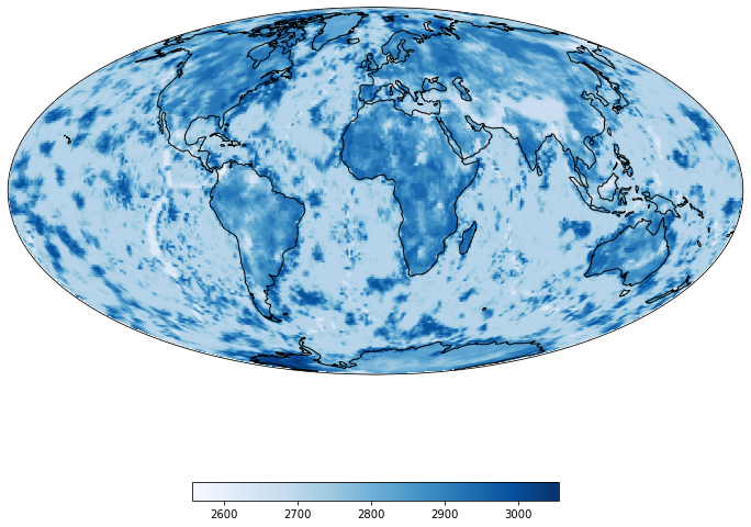
## make a global raster of some quantity

lonv, latv = np.meshgrid(np.linspace(-180,180,360), np.linspace(-90,90,180), sparse=False, indexing='xy')

l1 = litho.layer_depth(latv, lonv, "LID-BOTTOM")
l2 = litho.layer_depth(latv, lonv, "LID-TOP")

lthickness = (l1 - l2)*0.001

l1 = litho.layer_depth(latv, lonv, "CRUST3-BOTTOM")
l2 = litho.layer_depth(latv, lonv, "CRUST1-TOP")

cthickness = (l1 - l2)*0.001

# density at 1km depth
depths = np.ones_like(lonv, dtype=np.float)*5.0

ids, density_at_1km = litho.property_at_lat_lon_depth_points(latv, lonv, depths, quantity_ID="DENSITY")
/var/folders/g3/zs57lnv5087f66fcky707_ww0000gp/T/ipykernel_8290/1934221471.py:16: DeprecationWarning: `np.float` is a deprecated alias for the builtin `float`. To silence this warning, use `float` by itself. Doing this will not modify any behavior and is safe. If you specifically wanted the numpy scalar type, use `np.float64` here.
Deprecated in NumPy 1.20; for more details and guidance: https://numpy.org/devdocs/release/1.20.0-notes.html#deprecations
  depths = np.ones_like(lonv, dtype=np.float)*5.0
%matplotlib inline

import cartopy
# import gdal
import cartopy.crs as ccrs
import matplotlib.pyplot as plt

projection1 = ccrs.Orthographic(central_longitude=140.0, central_latitude=0.0, globe=None)
projection2 = ccrs.Mollweide(central_longitude=0)
base_projection = ccrs.PlateCarree()

global_extent     = [-180.0, 180.0, -90.0, 90.0]


fig = plt.figure(figsize=(12, 12), facecolor="none")
ax  = plt.subplot(111, projection=projection2)
ax.coastlines()
ax.set_global()

m = ax.imshow(density_at_1km.reshape(-1,360), origin='lower', transform=base_projection,
              extent=global_extent, zorder=0, cmap="Blues")

plt.colorbar(mappable=m, orientation="horizontal", shrink=0.5)
<matplotlib.colorbar.Colorbar at 0x13d66abe0>
def great_circle_profile(startlonlat, endlonlat, depths, resolution, QID):
    """
    model: self
    ll0: (lon0, lat0)
    ll1: (lon1, lat1)
    depths (km)
    resolution: separation (km) of locations to sample along the profile
    """

    import stripy

    lons, lats = great_circle_Npoints(np.radians(startlonlat), np.radians(endlonlat), 1000)

    ## Would be useful to have distance measure here to map resolutions ...

    data = np.empty( (lons.shape[0], depths.shape[0]))

    for s, ll in enumerate(lons):
        c, profile = litho.property_on_depth_profile(np.degrees(lats[s]), np.degrees(lons[s]), depths, QID)
        data[s,:] = profile[:]


    return np.degrees(lons), np.degrees(lats), data


def great_circle_Npoints(lonlat1, lonlat2, N):
    """
    N points along the line joining lonlat1 and lonlat2
    """

    ratio = np.linspace(0.0,1.0, N).reshape(-1,1)

    lonlat1r = np.radians(lonlat1)
    lonlat2r = np.radians(lonlat2)


    xyz1 = np.array(stripy.spherical.lonlat2xyz(lonlat1r[0], lonlat1r[1])).T
    xyz2 = np.array(stripy.spherical.lonlat2xyz(lonlat2r[0], lonlat2r[1])).T

    mids = ratio * xyz2 + (1.0-ratio) * xyz1
    norm = (mids**2).sum(axis=1)
    xyzN = mids / norm.reshape(-1,1)

    lonlatN = stripy.spherical.xyz2lonlat( xyzN[:,0], xyzN[:,1], xyzN[:,2])

    return np.degrees(lonlatN)
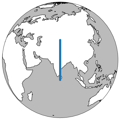
depths = np.linspace(-10.0, 250, 100)
startlonlat=np.array([80.0,5.0])
endlonlat  =np.array([80.0,45.0])

midlonlat = 0.5 * ( startlonlat + endlonlat)

lons, lats, d = great_circle_profile(startlonlat, endlonlat, depths, 2.5, "DENSITY")
lonlat1r = np.radians(startlonlat)
lonlat2r = np.radians(endlonlat)
xyz1 = np.array(stripy.spherical.lonlat2xyz(lonlat1r[0], lonlat1r[1])).T
xyz2 = np.array(stripy.spherical.lonlat2xyz(lonlat2r[0], lonlat2r[1])).T

N=100
ratio = np.linspace(0.0,1.0, N).reshape(-1,1)
mids = ratio * xyz2 + (1.0-ratio) * xyz1
fig = plt.figure(figsize=(7, 7), facecolor="none")

ax  = plt.subplot(111, projection=ccrs.Orthographic(central_latitude=midlonlat[1], central_longitude=midlonlat[0]))
ax.set_global()

ax.add_feature(cartopy.feature.OCEAN, alpha=1.0, facecolor="#BBBBBB", zorder=0)
ax.scatter(lons, lats, transform=ccrs.PlateCarree(), zorder=100)

ax.coastlines()
<cartopy.mpl.feature_artist.FeatureArtist at 0x13d7b4340>
# Compute some properties about the profile line itself
drange = depths[-1] - depths[0]
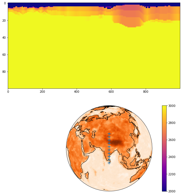
#
# Cross section
#
fig = plt.figure(figsize=(12, 12), facecolor="none")
ax = plt.subplot(211)
ax2 = plt.subplot(212, projection=ccrs.Orthographic(central_latitude=midlonlat[1],
central_longitude=midlonlat[0]))
image = d[:,:]
m1 = ax.imshow(image.T, origin="upper", cmap="plasma", aspect=5.0, vmin=2000, vmax=3000)
plt.colorbar(mappable=m1, )
#
# Map / cross section
#
ax2.set_global()
global_extent = [-180.0, 180.0, -90.0, 90.0]
m = ax2.imshow(cthickness, origin='lower', transform=ccrs.PlateCarree(),
extent=global_extent, zorder=0, cmap="Oranges")
ax2.add_feature(cartopy.feature.OCEAN, alpha=0.25, facecolor="#BBBBBB")
ax2.coastlines()
lonr, latr = great_circle_Npoints(np.radians(startlonlat), np.radians(endlonlat), 10)
ptslo = np.degrees(lonr)
ptsla = np.degrees(latr)
ax2.scatter (ptslo, ptsla, marker="+", s=100, transform=ccrs.PlateCarree(), zorder=101)
/var/folders/g3/zs57lnv5087f66fcky707_ww0000gp/T/ipykernel_8290/1179517594.py:17: MatplotlibDeprecationWarning: Starting from Matplotlib 3.6, colorbar() will steal space from the mappable's axes, rather than from the current axes, to place the colorbar.  To silence this warning, explicitly pass the 'ax' argument to colorbar().
  plt.colorbar(mappable=m1, )
<matplotlib.collections.PathCollection at 0x13d8c1e50>
Next example: Crust 1.0