
A quick look at the depth-age relationship for the seafloor.
Contents
A quick look at the depth-age relationship for the seafloor.
We can obtain the global (ocean) age grid from the University of Sydney Earthbyte Group (https://www.earthbyte.org/age-and-bathymetry-of-the-worlds-ocean-crust-for-the-last-140-million-years/). The data should look like this when plotted on a map.
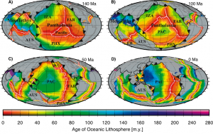
Note: I downloaded this file: age.3.6.nc which is “A short integer netCDF formatted file. The age units are in millions of years, multiplied by 100 (to enable storage as short The file spans longitudes from 0 E to 360 E and latitudes from 90 N to -90 N. 6 minute resolution, gridline-registered.”
The ftp site where this data is stored does not serve the data in a way that xarray can read but otherwise it should be similar to what we did for the topography / bathymetry data.
References
Müller, R.D., Sdrolias, M., Gaina, C. and Roest, W.R., 2008, Age spreading rates and spreading asymmetry of the world’s ocean crust, Geochemistry, Geophysics, Geosystems, 9, Q04006, doi:10.1029/2007GC001743
Read the data and make a plot
Let’s see if the data are what we expect given the Earthbyte image above.
We will need to import xarray to read the compressed file.
import xarray
import numpy as np

age_dataset = "../Data/age.3.6.nc"
age_data = xarray.open_dataset(age_dataset)
subs_data = age_data.sel(x=slice(-180,180, 1), y=slice(-90, 90, 1))

lons = subs_data.coords.get('x')
lats = subs_data.coords.get('y')
vals = subs_data['z']

x,y = np.meshgrid(lons.data, lats.data)
age = vals.data
import matplotlib.pyplot as plt
%matplotlib inline

import cartopy.crs as ccrs
import cartopy.feature as cfeature

map_extent = (-180, 180,-90,90)

coastline = cfeature.NaturalEarthFeature('physical', 'coastline', '10m',
                           edgecolor=(1.0,0.8,0.0),
                           facecolor="none")

plt.figure(figsize=(15, 10))
ax = plt.subplot(111, projection=ccrs.PlateCarree())
ax.set_extent(map_extent)

ax.add_feature(coastline, edgecolor="black", linewidth=0.5, zorder=3)

plt.imshow(age, extent=map_extent, transform=ccrs.PlateCarree(),
           cmap='RdYlBu', origin='lower', vmin=0.0, vmax=180.0)
<matplotlib.image.AxesImage at 0x1568dc5e0>
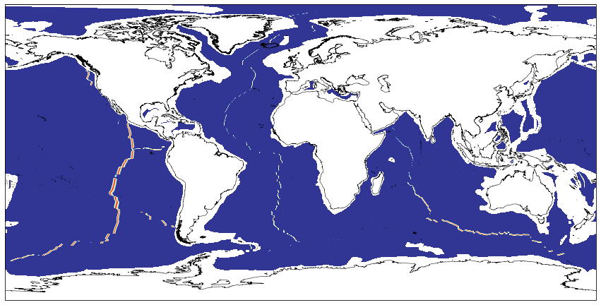
Is this correct ?
Well, it does not look quite right but do you think the data are scrambled or is something else wrong?
Debugging
Remember to read the description above. What is the range of age in the age array ? What do you expect for the Earth’s oceans ?
Hint; check the documentation for np.isnan()