Index
Contents
Index
Louis Moresi, louis.moresi@anu.edu.au
In this section, we take time to pull apart some common and useful packages that are used in the Geosciences. The idea is for you to start to forget that you are learning python and get caught up in some interesting applications.
Numpy and Scipy
numpy brings hard-core array data types into python with very efficient implementations of standard mathematical operators on arrays. It also manages to implement a collection of wildcards on array indices and array slices that make for very compact and tidy implementations (provided you understand the basic principles). numpy is a very good example of how python allows a programmer to expose their code at exactly the right level of detail for the user.
scipy is an eclectic collection of useful scientific routines that is critically dependent upon numpy.
The notebooks cover the basic data types in numpy and work through an example from the Game of Life which shows how to implement structured array operations in practice.
Once you think you have mastered numpy array indexing, have a look at the cartopy mapping examples which use numpy extensively to manipulate images and data arrays.
Plots and Maps and Images
The package matplotlib is a must-use in the ipython / jupyter world because it is pre-loaded into the notebook environment and is very easy to start using. The interface is clearly evolutionary rather than a ground-up intelligent design but it works … a quick intro notebook will get you started.
We will use the mapping package cartopy designed by the UK Met Office. cartopy takes advantage of matplotlib having implemented a generic coordinate-tranformation interface and builds in all of the common map projections. This is a remarkably simple concept that leads to some exceptionally powerful mapping capabilities. We work through a series of exercises to map raster data, contour scalar fields and display vector data on the Earth’s surface. cartopy has the capacity to plot maps from on-demand mapping services and is very well set up for careful registration of satellite imagery onto basemaps. See the example notebooks to get started and don’t forget to review the numpy tutorial before diving in.
Spherical triangulation and meshing
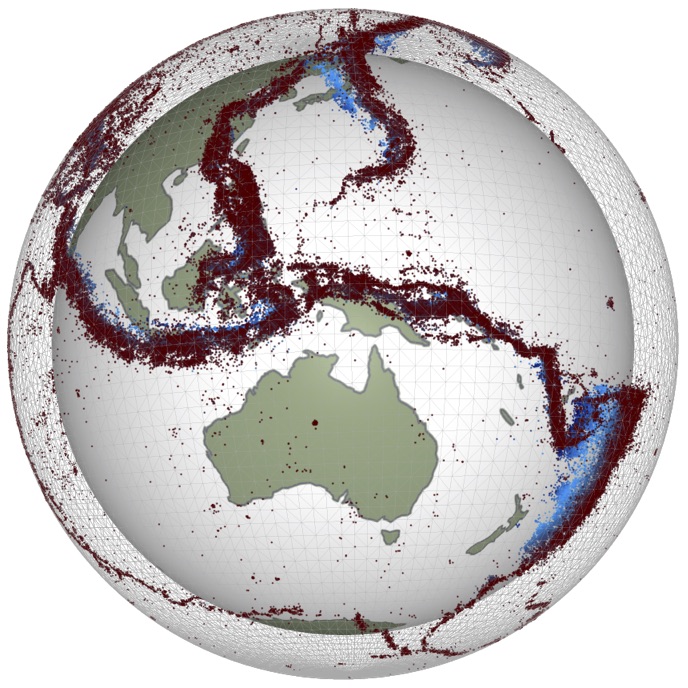
stripy is a package that builds Delaunay triangulations and Voronoi diagrams on the sphere. It is very useful for making refined triangular meshes, gridding Earth data, interpolating, finding gradients, making heat maps, and smoothing scattered data on the Earth’s surface. stripy also has am exactly matched Cartesian equivalent.
Index of the Spherical triangulation examples
Index of the Cartesian triangulation examples
Application: an interface to the litho 1.0 dataset which is a model that is based on a refined icosahedral mesh (trivial in
stripy)
Sympy
sympy is a symbolic algebra package built in python that has much in common with Mathematica or Maple but within the standard python language. If you dig deeper into sympy, you will find a very convoluted structure that (in my opinion) violates almost every design principle I am trying to teach you. Nevertheless, a very clever package that is also extremely useful.
The sample notebooks do not go very deep into sympy but should give you a flavour of how much work the object model of python can be made to do. It should also give you a hint that documentation and thoughtful design are critical in python where so much can be hidden.
Numerical Models
When we think of solving the partial differential equations that often form the basis of a mathematical model, we often think about how to find an exact, analytic solution as we did with sympy in the previous set of examples. However, another way to think about a model that can be represented by a PDE is that it consists of a number of gradients that are in balance with each other, with changes in the state of the system and with the boundary conditions. It may well be possible to find an exact solution but often it is not.
In calculus, we take limits of infinitessimal quantities to find the analytic form of derivatives but we can also gain a great deal of insight by simply examining the balances before taking the limit and from examining how those balances occur and they changes they drive. Typically, we do this with some numerical approach to keeping track of the changes on a grid of points from which we can store information and compute gradients in space and time. This is an field that is broad as well as deep and we will only scratch the surface in these examples.
