Non-dimensional equations & dimensionless numbers
$$ % Global LaTeX macros for MathJax
% Differential operators % Color commands (MathJax compatible)$$
Before too long it would be a good idea to get a feeling for the flavour of these equations which continual rearrangements will not do — it is necessary to examine some solutions.
First of all it is a good idea to make some simplifications based on the kinds of problems we will want to attack. The first thing to do, as is often the case when developing a model, is to test whether any of the terms in the equations are negligibly small, or dominant. To do this, we are going to need to have some physical insight into the kinds of problems we are going to solve - for example, some terms may be negligible for slow moving flow but not if the flow is fast (but what does ‘fast’ really mean ?)
One trick that is very common in fluid dynamics is to re-scale the equations using units that are in some way natural to the problem we are trying to solve. This helps us to answer the question that came up a moment ago: if a typical velocity is 1, then ‘slow’ is \(v \ll 1\) and ‘fast’ is when \(v \gg 1\).
Remember that even very rational systems of units like the SI system are still arbitrary and based on the scale of human experience: a metre is not far off the length of a step when we walk, a second is our heartbeat, carry a litre of water when you go walking.
We don’t need to define and name a whole new system of units any time we start analysing a new problem, but the fact that we could do this suggests there is a way to consider the scale of a problem independenly to the underlying character of the way things balance each other as the system changes through time.
What we can do is consider ‘typical values’ for the independent dimensions of a system (mass, length, time, temperature, that sort of thing) which can be used to rescale the standard units. For example, we might rescale all lengths by the size of the system we are studying, \(d\) (e.g. mantle thickness or depth of fluid in a lab tank), time according to the characteristic time for diffusion of heat over that distnace, and temperature by maximum temperature difference we observe at the start.
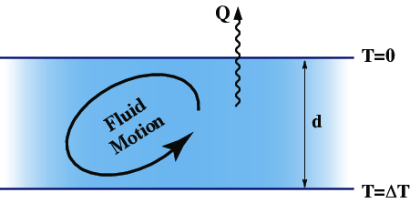
Various scalings result, with the new variables indicated using a prime (\('\)).
\[ \begin{array}{llll} x = d.x' & \partial / \partial x = (1/d) \partial / \partial x' & \nabla = (1/d) \nabla ' \\ t = (d^2/\kappa) t' & \partial / \partial t = (\kappa/d^2) \partial / \partial t' & \\ T = \Delta T T' & & \\ v = (\kappa / d) v' && \\ p= p_0 + (\eta \kappa / d^2) p' \end{array} \]
where \(\nabla p_0 = - g \rho_0\)
Substituting for all the existing terms in the Navier-Stokes equation (?eq-navstokes) using the equation of state for thermally induced variation in density (?eq-state) gives:
\[ \frac{\rho_0 \kappa}{d^2} \frac{D}{Dt'} \left( \frac{\kappa}{d} \mathbf{v}' \right) = \frac{\eta}{d^2} \acute{\nabla}^2 \left( \frac{\kappa}{d} \mathbf{v}' \right) - \frac{\eta \kappa}{d^3} \acute{\nabla} p' + g \rho_0 \alpha \Delta T T' \hat{\mathbf{z}} \]
Collecting everything together gives
\[ \frac{\rho_0 \kappa^2}{d^3} \frac{D\mathbf{v}'}{Dt'} = \frac{\eta \kappa}{d^3} \acute{\nabla}^2 \mathbf{v}' - \frac{\eta \kappa}{d^3} \acute{\nabla} p' + g \rho_0 \alpha \Delta T T' \hat{\mathbf{z}} \]
Divide throughout by \(\eta \kappa / d^3\) gives
\[ \begin{aligned} \frac{\rho \kappa}{\eta} \frac{D\mathbf{v}'}{Dt'} & = \acute{\nabla}^2 \mathbf{v}' - \acute{\nabla} p' + \frac{g \rho_0 \alpha \Delta T d^3}{\kappa \eta} T' \hat{\mathbf{z}} \nonumber \\ \textrm{or} \;\;\; \frac{1}{{\rm Pr}} \frac{D\mathbf{v}'}{Dt'} & = \acute{\nabla}^2 \mathbf{v}' - \acute{\nabla} p' + {\rm Ra} T' \hat{\mathbf{z}} \end{aligned} \]
\(\rm Pr\) is known as the Prandtl number, and \(\rm Ra\) is known as the Rayleigh number; both are non-dimensional numbers. By choosing to scale the equations (and this is still perfectly general as we haven’t forced any particular choice of scaling yet), we have condensed the different physical variable quantities into just two numbers. The benefit of this procedure is that it tells us how different quantities trade off against one another. For example, we see that if the density doubles, and the viscosity doubles, then the solution should remain unchanged.
In fact, the main purpose of this particular exercise is about to be revealed. The value of mantle viscosity is believed to lie somewhere between \(10^{19}\) and \(10^{23}\) \({\rm Pa . s}\), the thermal diffusivity is around \(10^{-6}{\rm m}^2{\rm s}^{-1}\), and density around \(3300 {\rm kg . m}^{-3}\). This gives a Prandtl number greater than \(10^{20}\). Typical estimates for the Rayleigh number are between \(10^6\) and \(10^8\) depending on the supposed depth of convection, and the uncertain mantle viscosity.
Obviously, the time-dependent term can be neglected for the mantle, since it is at least twenty orders of magnitude smaller than other terms in the equations. The benefit of this is that the nasty advection term for momentum is eliminated – flow in the mantle is at the opposite extreme to turbulent flow. The disadvantage is that the equations now become non-local: changes in the stress field are propogated instantly from point to point which can make the equations a lot harder to solve. This can be counter-intuitive but the consequences are important when considering the dynamic response of the Earth to changes in, for example, plate configurations.
Incidentally, a third, independent dimensionless number can be derived for the thermally driven flow equations. This is the Nusselt number
\[ {\rm Nu} = \frac{Q}{k\Delta T} \]
and is the ratio of actual heat transported by fluid motions in the layer compared to that transported conductively in the absence of fluid motion.
All other dimensionless quantities for this system can be expressed as some combination of the Nusselt, Rayleigh and Prandtl numbers. The Prandtl number is a property of the fluid itself – typical values are: air, $$1; water, \(\sim\) 6; non-conducting fluids \(10^3\) or more; liquid metal, $$0.1. Rayleigh number and Nusselt number are both properties of the chosen geometry.
The stream function
For incompressible flows in two dimensions it can be very convenient to work with the stream-function – a scalar quantity which defines the flow everywhere. The stream function is the scalar quantity,\(\psi\), which satisfies
\[ v_1 = -\frac{\partial \psi}{\partial x_2} \mbox{\hspace{1cm}} v_2 = \frac{\partial \psi}{\partial x_1} \tag{11.1}\]
so that, automatically,
\[ \frac{\partial v_1}{\partial x_1} + \frac{\partial v_2}{\partial x_2} = 0 \]
Importantly, computing the following
\[ (\mathbf{v} \cdot \nabla) \psi = v_1 \frac{\partial \psi}{\partial x_1} + v_2 \frac{\partial \psi}{\partial x_2} = \frac{\partial \psi}{\partial x_2} \frac{\partial \psi}{\partial x_1} - \frac{\partial \psi}{\partial x_1} \frac{\partial \psi}{\partial x_2} = 0 \]
tells us that \(\psi\) does not change due to advection – in other words, contours of constant \(\psi\) are streamlines of the fluid.
Provided we limit ourselves to the xy plane, it is possible to think of equation (Equation 11.1) as
\[ \mathbf{v} = \nabla \times (\psi \hat{\mathbf{k}}) \]
This form can be used to write down the 2D axisymetric version of equation (Equation 11.1)
\[ \begin{aligned} u_r = -\frac{1}{r}\frac{\partial \psi}{\partial \theta} & & u_\theta = \frac{\partial \psi}{\partial r} \end{aligned} \]
which automatically satisfies the incompressibility condition in plane polar coordinates \[ \frac{1}{r}\frac{\partial}{\partial r}(ru_r) + \frac{1}{r}\frac{\partial u_\theta}{\partial \theta} = 0 \]
Vorticity
Vorticity is defined by \[ \boldsymbol{\omega} = \nabla \times \mathbf{v} \]
In 2D, the vorticity can be regarded as a scalar as it has only one component which lies out of the plane of the flow.
\[ \omega = \frac{\partial v_2}{\partial x_1} - \frac{\partial v_1}{\partial x_2} \]
which is also exactly equal to twice the local measure of the spin in the fluid. Local here means that it applies to an infinitessimal region around the sample point but not to the fluid as a whole.
This concept is most useful in the context of invicid flow where vorticity is conserved within the bulk of the fluid provided the fluid is subject to only conservative forces – that is ones which can be described as the gradient of a single-valued potential.
In the context of viscous flow, the viscous effects acts cause diffusion of vorticity, and in our context, the fact that buoyancy forces result from to (irreversible) heat transport means that vorticity has sources. Taking the curl of the Navier-Stokes equation, and substituting for the vorticity where possible gives
\[ \frac{1}{\rm Pr} \left( \frac{D \boldsymbol{\omega}}{D t} - (\boldsymbol{\omega} \cdot \nabla) \mathbf{v} \right) = \eta \nabla ^2 \boldsymbol{\omega} + {\rm Ra} \frac{\partial T}{\partial x_1} \]
The pressure drops out because \(\nabla \times \nabla P = 0 \mbox{\hspace{0.5cm}} \forall P\).
Stream-function, vorticity and the biharmonic equation
In the context of highly viscous fluids in 2D, the vorticity equation is
\[ \nabla ^2 \omega = - Ra \frac{\partial T}{\partial x_1} \tag{11.2}\]
and, by considering the curl of \((-\partial \psi / \partial x_2, \partial \psi / \partial x_1, 0)\) the stream function can be written
\[ \nabla ^2 \psi = \omega \tag{11.3}\]
This form is useful from a computational point of view because it is relatively easy to solve the Laplacian, and the code can be reused for each application of the operator. The Laplacian is also used for thermal diffusion – one subroutine for three different bits of physics which is elegant in itself if nothing else.
The biharmonic operator is defined as
\[ \nabla^4 \equiv \nabla^2 ( \nabla ^2) \equiv \left( \frac{\partial ^4}{\partial x_1^4} + \frac{\partial ^2}{\partial x_1^2} \frac{\partial ^2}{\partial x_2^2} + \frac{\partial ^4}{\partial x_2^4} \right) \]
The latter form being the representation in Cartesian coordinates.
Using this form, it is easy to show that equations (Equation 11.2) and (Equation 11.3) can be combined to give
\[ \nabla^4 \psi = -{\rm Ra} \frac{\partial T}{\partial x_1} \tag{11.4}\]
Poloidal/Toroidal velocity decomposition
The stream-function / vorticity form we have just used is a simplification of the more general case of the poloidal / toroidal velocity decomposition which turns out to be useful when we want to understand the balance of different contributions to the governing equation.
We can make a Helmholtz decomposition of the velocity vector field:
\[ \mathbf{u} = \nabla \phi + \nabla \times \mathbf{A} \]
Then for an incompressible flow, since \(\nabla \cdot \mathbf{u} = 0\), \[ \mathbf{u} = \nabla \times \mathbf{A} \tag{11.5}\]
Now suppose there is some direction (\(\hat{\mathbf{z}}\)) which we expect to be physically favoured in the solutions, we can rewrite Equation 11.5 as
\[ \mathbf{u} = \textcolor[rgb]{0.7,0.0,0.0}{\nabla \times(\Psi \hat{\mathbf{z}})} + \textcolor[rgb]{0.0,0.0,0.7}{ \nabla \times\nabla \times(\Phi \hat{\mathbf{z}})} \tag{11.6}\]
Where the first term on the right is the Toroidal part of the flow, and the second term is the Poloidal part. Why is this useful ? Let’s substitute (Equation 11.6) into the Stokes’ equation for a constant viscosity fluid
\[ \eta \nabla^2 \mathbf{u} - \nabla p = g \rho \hat{\mathbf{z}} \tag{11.7}\]
where \(\hat{\mathbf{z}}\) is the vertical unit vector (defined by the direction of gravity) and is clearly the one identifiable special direction, then equate coefficients in the \(\hat{\mathbf{z}}\) direction, and using the following results:
\[ \hat{\mathbf{z}} \cdot \nabla \times \nabla^2 \mathbf{u} = - \nabla^2 \nabla_h^2\Psi \]
\[ \hat{\mathbf{z}} \cdot \nabla \times \nabla \times \nabla^2 \mathbf{u} = \nabla^2 \nabla^2 \nabla_h^2\Phi \]
where
\[ \nabla_h = \left( \frac{\partial}{\partial x}, \frac{\partial}{\partial y}, 0 \right) \]
is a gradient operator limited to the plane perpendicular to the special direction, \(\hat{\mathbf{z}}\).
If we first take the curl of (Equation 11.7), and look at the \(\hat{\mathbf{z}}\) direction,
\[ \hat{\mathbf{z}} \cdot \eta \nabla \times \nabla^2 \mathbf{u} = -\eta \nabla^2 \nabla_h^2\Psi = \hat{\mathbf{z}} \cdot \left( g \nabla \times \left( \rho \hat{\mathbf{z}}\right)\right) = 0 \]
we see that there is no contribution of the toroidal velocity field to the force balance. This balance occurs entirely through the poloidal part of the velocity field. If we take the curl twice and, once again, look at the \(\hat{\mathbf{z}}\) direction:
\[ \hat{\mathbf{z}} \cdot \eta \nabla \times \nabla \times \nabla^2 \mathbf{u} = \eta \nabla^2 \nabla^2 \nabla_h^2 \Phi = \hat{\mathbf{z}} \cdot g \nabla \times \nabla \times \left( \rho \hat{\mathbf{z}}\right) = \nabla_h^2 (\rho g) \]
Which is the 3D equivalent of the biharmonic equation that we derived above.
Note: if the viscosity varies in the \(\hat{\mathbf{z}}\) direction, then this same decoupling still applies: bouyancy forces do not drive any toroidal flow. Lateral variations in viscosity (perpendicular to \(\hat{\mathbf{z}}\)) couple the buoyancy to toroidal motion. This result is general in that it applies to the spherical geometry equally well assuming the radial direction (of gravity) to be special.
Exercises
This exercises section is newly added as a placeholder for future content. These exercises are currently conceptual prompts that need to be developed with detailed problem statements, worked examples, and solutions.
Changes made: - Created 5 placeholder exercises aligned with chapter content - Added 1 worked solution for stream function properties - Exercises need expansion with numerical values and step-by-step guidance - Additional exercises should be added covering: dimensional analysis, scaling laws, corner flow details
Exercises marked with ⭐ have worked solutions provided. Additional exercises will be added as the chapter develops.
Exercise 1: Non-dimensionalizing the Stokes Equation
Starting from the dimensional Stokes equation, derive the non-dimensional form showing all intermediate steps. Identify where the Rayleigh number appears and explain its physical significance.
Exercise 2: Poloidal-Toroidal Decomposition
For the velocity field in spherical coordinates:
Show that any solenoidal (divergence-free) vector field can be decomposed into poloidal and toroidal components
Explain why toroidal flow cannot generate buoyancy-driven convection
Give examples of geophysical flows that are predominantly toroidal
Exercise 3: Estimating Mantle Rayleigh Numbers
Using typical mantle values, calculate the Rayleigh number for:
- Whole mantle convection
- Upper mantle only convection
- Thermal boundary layer at the CMB (use appropriate length scale)
Compare your results and discuss the implications for convection vigor.
Exercise 4: Stream Function Properties ⭐
For 2D incompressible flow, the stream function \(\psi\) is defined such that: \[ u = \frac{\partial \psi}{\partial y}, \quad v = -\frac{\partial \psi}{\partial x} \]
Show that this automatically satisfies incompressibility
Demonstrate that streamlines are curves of constant \(\psi\)
Show that the volume flux between two streamlines equals the difference in \(\psi\) values
Exercise 5: Corner Flow Solution
Examine the corner flow solution for subduction zones:
Verify that the given velocity field satisfies incompressibility
Calculate the strain rate tensor for this flow
Where is the maximum strain rate located?
How does the solution change with the dip angle of the subducting slab?
Solutions to Selected Exercises
(a) Incompressibility:
The divergence of the velocity field is: \[ \nabla\cdot\mathbf{u}= \frac{\partial u}{\partial x} + \frac{\partial v}{\partial y} = \frac{\partial^2 \psi}{\partial x \partial y} - \frac{\partial^2 \psi}{\partial y \partial x} = 0 \]
The mixed partial derivatives are equal (Schwarz’s theorem), so incompressibility is automatically satisfied.
(b) Streamlines:
A streamline is tangent to the velocity vector at every point: \[ \frac{dy}{dx} = \frac{v}{u} \]
Along a curve of constant \(\psi\): \[ d\psi = \frac{\partial \psi}{\partial x}dx + \frac{\partial \psi}{\partial y}dy = -v\,dx + u\,dy = 0 \]
Therefore: \(\frac{dy}{dx} = \frac{v}{u}\), confirming that lines of constant \(\psi\) are streamlines.
(c) Volume flux:
The volume flux through a curve from point A to point B is: \[ Q = \int_A^B \mathbf{u}\cdot \hat{\mathbf{n}} \, ds \]
where \(\hat{\mathbf{n}}\) is the normal to the curve. Using the stream function definition and Stokes’ theorem, this equals: \[ Q = \psi_B - \psi_A \]
The volume flux between streamlines is simply the difference in their \(\psi\) values.