Example: Using Citations and Math

This chapter demonstrates how to use citations and mathematics in the book, showing both the source markup and the rendered output.

For complete documentation, see the Quarto Documentation and specifically:

• Equations
• Citations
• Cross-references

Citations

Source Markup

For a comprehensive introduction to geodynamics, see @turcotte2014.
The numerical methods for mantle convection are well described in @zhong2007.

Multiple citations can be grouped: [@moresi1995; @moresi1996; @tackley2008].

For fluid dynamics fundamentals, classic texts include @batchelor1967 and @acheson1990.

Rendered Output

For a comprehensive introduction to geodynamics, see Turcotte and Schubert (2014). The numerical methods for mantle convection are well described in Zhong, Yuen, and Moresi (2007).

Multiple citations can be grouped: (L. Moresi and Solomatov 1995; L. N. Moresi, Zhong, and Gurnis 1996; Tackley 2008).

For fluid dynamics fundamentals, classic texts include Batchelor (1967) and Acheson (1990).

Mathematics with Proper Rendering

$$ % Global LaTeX macros for MathJax

% Differential operators % Color commands (MathJax compatible)

$$

Inline Math

Source Markup

The Stokes equation for incompressible flow is $\DIV \sigma = \rho \mathbf{g}$
where $\sigma$ is the stress tensor and $\rho$ is density.

Rendered Output

The Stokes equation for incompressible flow is \(\nabla\cdot\sigma = \rho \mathbf{g}\) where \(\sigma\) is the stress tensor and \(\rho\) is density.

Display Equations with Labels

Source Markup

$$
\DIV \sigma + \rho \mathbf{g} = 0
$$ {#eq-stokes-momentum}

$$
\DIV \uv = 0
$$ {#eq-incompressible}

We can reference equations: The momentum equation @eq-stokes-momentum
combined with incompressibility @eq-incompressible forms the basis of
mantle convection modeling.

Rendered Output

\[ \nabla\cdot\sigma + \rho \mathbf{g} = 0 \tag{23.1}\]

\[ \nabla\cdot\mathbf{u}= 0 \tag{23.2}\]

We can reference equations: The momentum equation Equation 23.1 combined with incompressibility Equation 23.2 forms the basis of mantle convection modeling.

Multi-line Equations

Source Markup

$$
\begin{aligned}
\frac{\partial T}{\partial t} + \uv \cdot \GRAD T &= \kappa \nabla^2 T + H \\
\DIV \uv &= 0 \\
\rho &= \rho_0(1 - \alpha T)
\end{aligned}
$$ {#eq-thermal-system}

Rendered Output

\[ \begin{aligned} \frac{\partial T}{\partial t} + \mathbf{u}\cdot \nabla T &= \kappa \nabla^2 T + H \\ \nabla\cdot\mathbf{u}&= 0 \\ \rho &= \rho_0(1 - \alpha T) \end{aligned} \tag{23.3}\]

The thermal convection system Equation 23.3 couples temperature and velocity.

Colored Math (for emphasis)

Source Markup

The $\Red{red}$ terms represent heating, while $\Blue{blue}$ terms represent cooling:

$$
\frac{\partial T}{\partial t} + \uv \cdot \GRAD T = \kappa \nabla^2 T + \Red{H} - \Blue{L}
$$

Rendered Output

The \({\color{red} red}\) terms represent heating, while \({\color{blue} blue}\) terms represent cooling:

\[ \frac{\partial T}{\partial t} + \mathbf{u}\cdot \nabla T = \kappa \nabla^2 T + {\color{red} H} - {\color{blue} L} \]

Figures

Source Markup

![Consider the fluid motions in a layer of arbitrary depth, $d$. The fluid is
assumed to have constant properties such as viscosity, thermal expansivity,
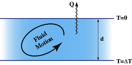thermal diffusivity.](../Images/Diagrams/layer.png){#fig-layer-example width=350px}

As shown in @fig-layer-example, the layer has depth $d$.

Rendered Output

Figure 23.1: Consider the fluid motions in a layer of arbitrary depth, \(d\). The fluid is assumed to have constant properties such as viscosity, thermal expansivity, thermal diffusivity.

As shown in Figure 23.1, the layer has depth \(d\).

Code Blocks

Python Code (Display Only)

Source Markup

```python
import numpy as np

def rayleigh_number(rho, g, alpha, delta_T, d, kappa, eta):
    """Calculate Rayleigh number for thermal convection."""
    return (rho * g * alpha * delta_T * d**3) / (kappa * eta)
```

Rendered Output

import numpy as np

def rayleigh_number(rho, g, alpha, delta_T, d, kappa, eta):
    """Calculate Rayleigh number for thermal convection."""
    return (rho * g * alpha * delta_T * d**3) / (kappa * eta)

Interactive Python (using pyodide)

Source Markup

```{pyodide-python}
import numpy as np
import matplotlib.pyplot as plt

# Calculate Rayleigh number for different viscosities
eta_values = np.logspace(19, 23, 50)
Ra = 3300 * 10 * 3e-5 * 3000 * (2900e3)**3 / (1e-6 * eta_values)

plt.figure(figsize=(8, 5))
plt.loglog(eta_values, Ra)
plt.xlabel('Viscosity (Pa·s)')
plt.ylabel('Rayleigh Number')
plt.title('Mantle Rayleigh Number vs Viscosity')
plt.grid(True, alpha=0.3)
plt.show()
```

Rendered Output

Using Global Macros

Source Markup

At the top of your file, include the math preamble:

::: {.hidden}
$$
% Global LaTeX macros for MathJax
\newcommand{\dGamma}{\mathbf{d}\boldsymbol{\Gamma}}
\newcommand{\uv}{\mathbf{u}}
\newcommand{\vv}{\mathbf{v}}
\newcommand{\nhat}{\mathbf{\hat{n}}}
\newcommand{\DIV}{\nabla\cdot}
\newcommand{\GRAD}{\nabla}
\newcommand{\CURL}{\nabla\times}
\DeclareMathOperator{\erfc}{erfc}

% Differential operators
\newcommand{\DDt}[1]{\frac{D #1}{D t}}
\newcommand{\ddt}[1]{\frac{d #1}{d t}}
\newcommand{\ppt}[1]{\frac{\partial #1}{\partial t}}
\newcommand{\ppx}[1]{\frac{\partial #1}{\partial x}}

% Color commands (MathJax compatible)
\newcommand{\Red}[1]{{\color{red} #1}}
\newcommand{\Green}[1]{{\color{green} #1}}
\newcommand{\Blue}[1]{{\color{blue} #1}}
\newcommand{\Emerald}[1]{{\color{teal} #1}}
$$
:::

Then use the defined macros:

- Velocity: $\uv$ or $\vv$
- Divergence: $\DIV \uv = 0$
- Gradient: $\GRAD T$
- Curl: $\CURL \mathbf{B}$
- Colored text: $\Red{important}$, $\Blue{cold}$, $\Green{check}$

Rendered Output

Available macros (already included at the top of this page):

• Velocity: \(\mathbf{u}\) or \(\mathbf{v}\)
• Divergence: \(\nabla\cdot\mathbf{u}= 0\)
• Gradient: \(\nabla T\)
• Curl: \(\nabla\times\mathbf{B}\)
• Colored text: \({\color{red} important}\), \({\color{blue} cold}\), \({\color{green} check}\)

Callout Blocks

Callout blocks are useful for highlighting important information, tips, warnings, and notes. See the Quarto Callout Blocks documentation for more details.

Source Markup

:::{.callout-note}
## Note Title (optional)

This is a note callout. Use it for general information that readers should be aware of.
:::

:::{.callout-tip}
## Tip: Numerical Stability

When implementing finite difference schemes, always check the CFL condition:
$$
\Delta t \leq \frac{\Delta x^2}{2\kappa}
$$
:::

:::{.callout-warning}
## Warning

The Boussinesq approximation breaks down when density variations exceed
approximately 10% of the reference density.
:::

:::{.callout-important}
## Important: Sign Conventions

In this book, we use the convention that tensile stress is positive and
compressive stress is negative.
:::

:::{.callout-caution}
## Caution: Computational Cost

Three-dimensional calculations can be extremely expensive. A grid with
$100^3$ points requires solving systems with ~1 million unknowns.
:::

Rendered Output

NoteNote Title (optional)

This is a note callout. Use it for general information that readers should be aware of.

TipTip: Numerical Stability

When implementing finite difference schemes, always check the CFL condition: \[ \Delta t \leq \frac{\Delta x^2}{2\kappa} \]

WarningWarning

The Boussinesq approximation breaks down when density variations exceed approximately 10% of the reference density.

ImportantImportant: Sign Conventions

In this book, we use the convention that tensile stress is positive and compressive stress is negative.

CautionCaution: Computational Cost

Three-dimensional calculations can be extremely expensive. A grid with \(100^3\) points requires solving systems with ~1 million unknowns.

Collapsible Callouts

You can make callouts collapsible (closed by default):

Source Markup

:::{.callout-note collapse="true"}
## Derivation Details (click to expand)

Here's the detailed derivation that advanced readers might want to see,
but beginners can skip:

Starting from the continuity equation...
[lengthy derivation]
:::

Rendered Output

NoteDerivation Details (click to expand)

Here’s the detailed derivation that advanced readers might want to see, but beginners can skip:

Starting from the continuity equation, we apply the divergence theorem and integrate by parts to obtain the weak formulation…

References

The bibliography will appear at the end of the book automatically based on all cited works.

Acheson, D. J. 1990. Elementary Fluid Dynamics. Oxford University Press.

Batchelor, G. K. 1967. An Introduction to Fluid Dynamics. Cambridge University Press.

Moresi, L. N., S. Zhong, and M. Gurnis. 1996. “The Accuracy of Finite Element Solutions of Stokes’ Flow with Strongly Varying Viscosity.” Physics of the Earth and Planetary Interiors 97 (1-4): 83–94.

Moresi, L., and V. Solomatov. 1995. “Numerical Investigation of 2D Convection with Extremely Large Viscosity Variations.” Physics of Fluids 7 (9): 2154–62.

Tackley, P. J. 2008. “Modelling Compressible Mantle Convection with Large Viscosity Contrasts in a Three-Dimensional Spherical Shell Using the Yin-Yang Grid.” Physics of the Earth and Planetary Interiors 171 (1-4): 7–18.

Turcotte, D., and G. Schubert. 2014. Geodynamics. 3rd ed. Cambridge University Press.

Zhong, S., D. A. Yuen, and L. N. Moresi. 2007. Numerical Methods for Mantle Convection. Treatise on Geophysics. Vol. 7.