Probing Planetary Interiors 2
July 1, 2025
Probing Planetary Interiors
How do we know what is inside a planet ?
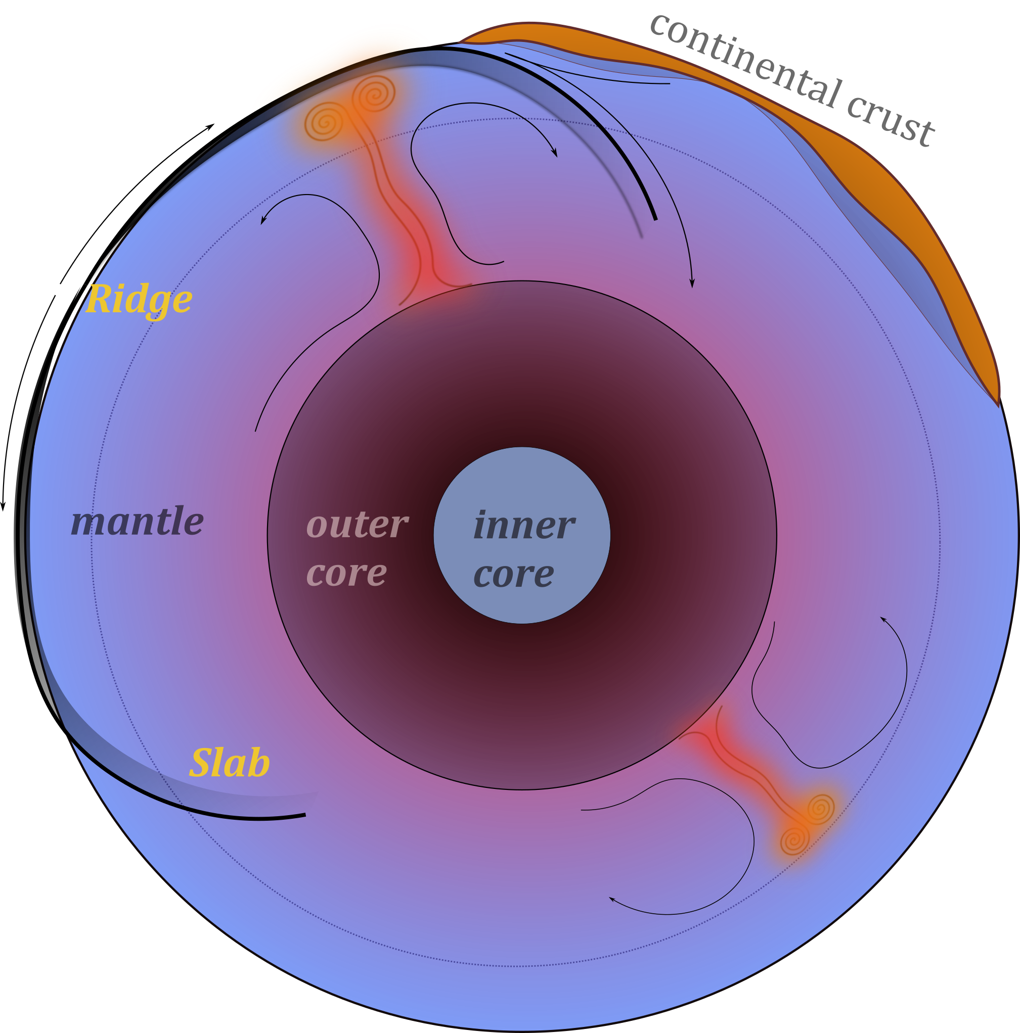
The circulation currents in the solid mantle move at a few cm/yr and plate motions are part of the overall circulation. On a global scale, movement is slow and viscous, especially in the deep mantle.
Mantle Plumes are also part of the overall circulation but much smaller than the slabs because they are cylindrical rather than sheets. Flow in the mantle is broad scale - small structures induce broad flow.
Other solid planets should follow the same basic physical models as the Earth, so it’s best to learn how things work on the most-instrumented planet first of all.
Mantle Convection
Convection in Earth’s interior is (a little bit) like a boiling pot (as we saw in a previous lecture)
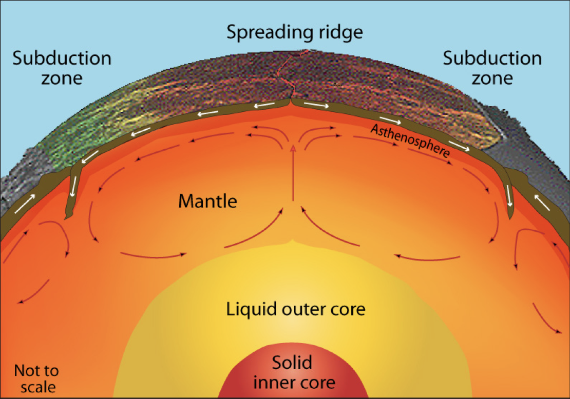
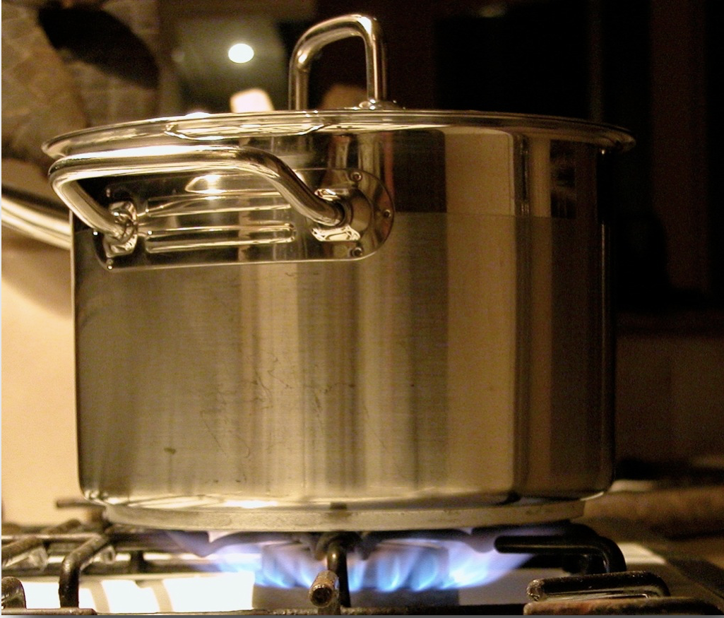
The hot soup rises to the surface, spreads and begins to cool, and then sinks back to the bottom of the pot where it is reheated and rises again. Why does hot soup rise and cold soup sink ?
General Observations on Convection
Without being particularly quantitative:
- Hot liquid is more buoyant than cold material and it tends to rise
- Cooler liquid is less buoyant and therefore tends to sink
- This can only happen if the two can move past each other
- Convection produces a self-stirring
Buoyancy forces are at work and viscous forces counteract these forces once the fluid is moving
\[ \textrm{buoyancy} \propto g \rho_0 \alpha(1-\Delta T) \]
Convection like this will only work when the soup is heated from below or, in the case of the Earth, if it is heated from within by radioactivity. (Can you see why) ?
Heat Transfer
Other ways that heat can be transferred include radiation, advection, and conduction.
Advection of heat is where some object carries an excess (or defecit of) heat energy from place to place.
Conduction is the transfer of heat (or electric current) from one substance to another by direct contact (lattice vibrations / electrons).
Radiation is the transfer of heat energy by photons that pass between two materials. It does not require any physical contact or indermediary material (e.g. it is not a problem to transfer heat across a vacuum this way).
![]()
Conduction & Fourier’s Law - i
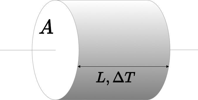
Fourier’s Law tells us how much heat, \(Q\) is conducted through a sample in a unit time
\[ Q=-\frac{k A \Delta T}{L} \]
\(A\) is the cross sectional area of the sample, \(L\) is its length, \(k\) is a thermal conductivity “constant” dependent on the nature of the material and often also on the temperature, and \(\Delta T\) is the temperature difference across the sample. (Note the minus sign because heat will always flow from a higher temperature to a lower temperature.)
Conduction & Fourier’s Law - ii
Fourier’s Law is explained using a simple thought experiment such as this one but it actually refers to the fact that heat flows down a temperature gradient.
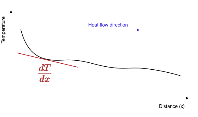
\[ q = - k \frac{dT}{dx} \]
\(q, (W/m^2)\) is called the heat flux and measures the flow of heat per unit area perpendicular to the temperature gradient
Conduction & Fourier’s Law - iii
If the heat flux into a region is not balanced by the heat flux out, the region must change temperature. For example, if more heat flow into a region than is flowing out, it will become warmer.
The heat flow in the diagram is away (in both directions) from the high temperature to the cooler areas. The loss of heat from this region is balanced by a reduced temperature.
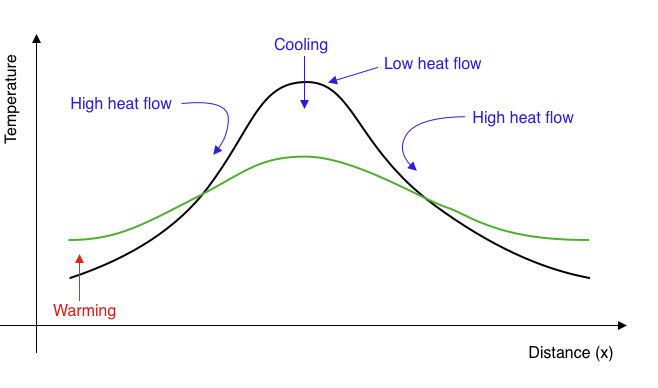
This process reduces the amplitude of temperature variations over time and makes the temperature smoother. Temperature extremes become smaller, gradients become lower, the heat flux everywhere becomes smaller: the temperature differences decay through time.
Newton’s Law of Cooling
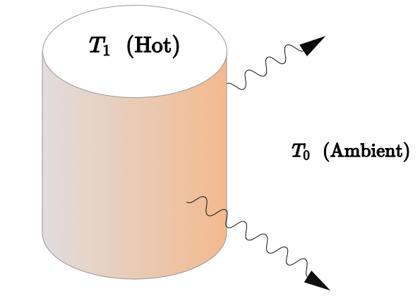
Another example of “thermal decay” occurs when we have a hot body in a cool environment loosing heat through its surface according to the Fourier Law.
The heat flux is proportional to the difference in temperature between the hot object and the surroundings, so
\[ \frac{dT}{dt} \propto T - T_0 \quad \rightarrow \quad T = T_1 e^{-\lambda t} \]
This is exactly the same equation for the anomalous temperature as for the quantity of a radioactive isotope remaining after a certain time and has the same solution with \(\lambda\) a constant for a particular experiment.
Solution for the uniform conduction of heat out of a sphere
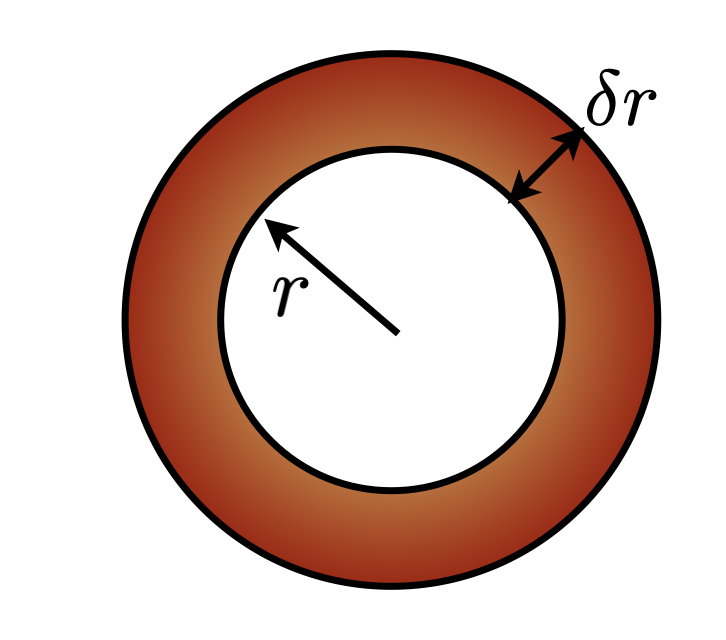
What is the equilibrium heat flow across a thin spherical shell ?
- Heat flux in balances heat flux out
- Account for heat generation within the shell
\[ Q_r = 4\pi r^2 \cdot q_r(r) \]
\[ Q_{r+\delta r} = 4\pi (r+\delta_r)^2 \cdot q_r(r+\delta_r) \]
The steady solution has this form
\[ T = -\frac{\rho H}{6 k} r^2 + \frac{C_1}{r} + C_2 \]
Which is only interesting if there is internal heating (\(H\)) and otherwise implies constant temperature / no additional heat at depth. Steady-state, of course, tells us nothing about the age of the Earth. \(C_1\) has to be zero, for the solution to be meaningful at \(r=0\).
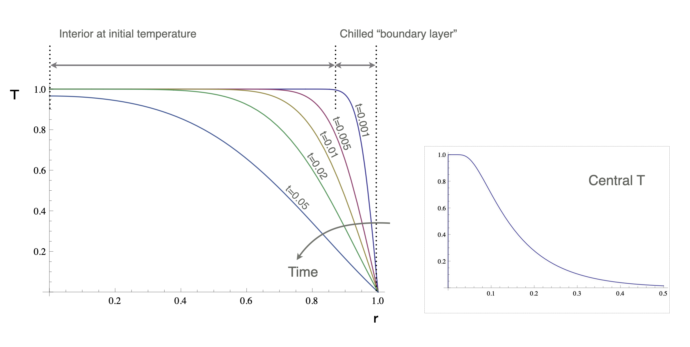
Transient solution for a sphere cooling from a uniform T
\[ T(r,t) = \frac{2}{r} \sum_{n=1}^{\infty} \exp\left( n^2\pi^2 t \right) \sin(n\pi r) \cdot \left( \frac{\sin(n\pi) - n \pi \cos(n\pi)}{n^2 \pi^2} \right) \]
Transient solution for a sphere cooling from a uniform T
\[ \frac{\partial T}{\partial r}(1,t) = -\sum_{n=1}^{\infty} \frac{2 e^{-n^2\pi^2 t} \left( n\pi \cos(n\pi) -\sin(n\pi) \right)^2}{n^2 \pi^2} \]
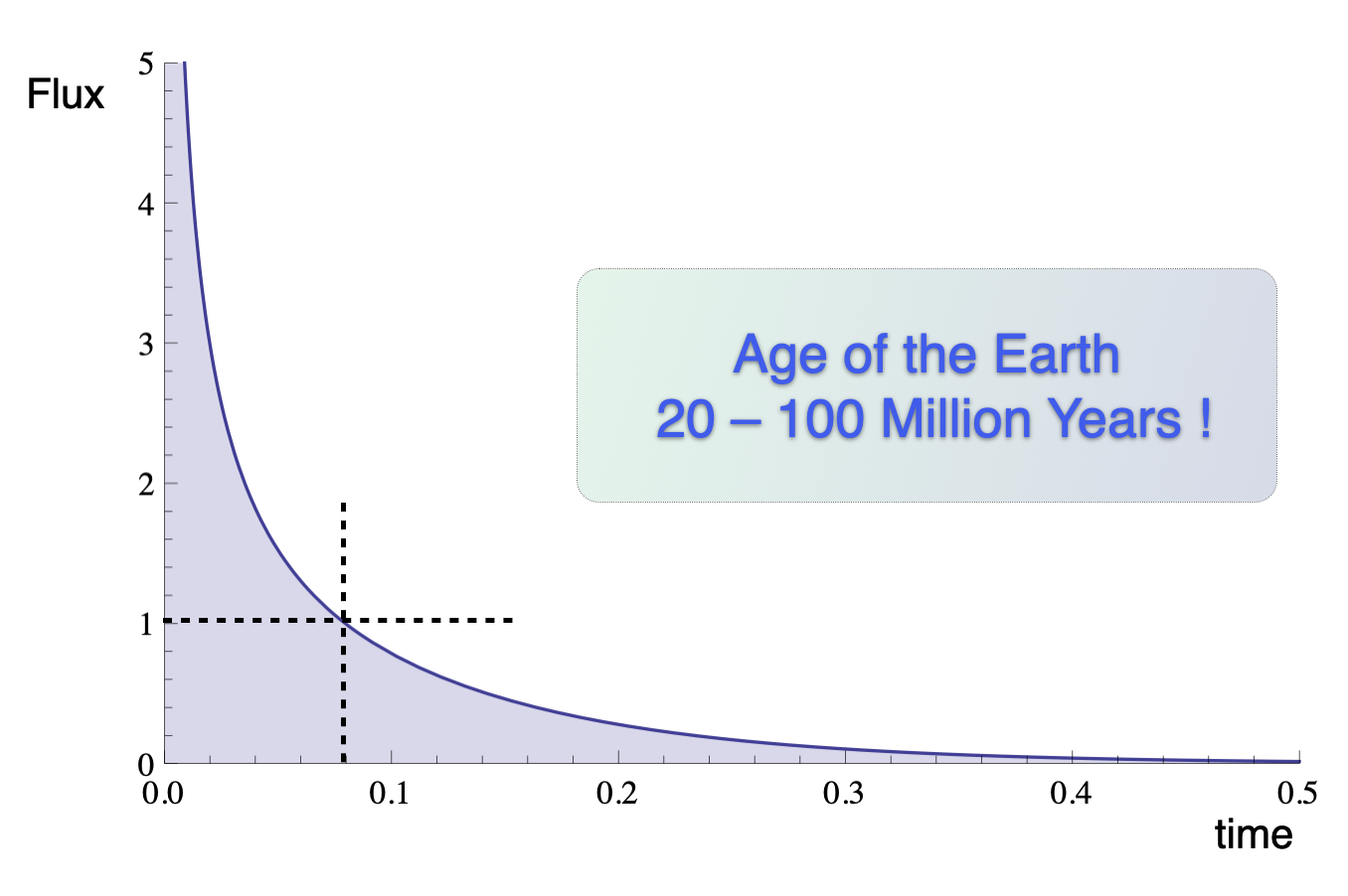
This is, essentially, the simplest version of estimate by Lord Kelvin for the age of the Earth based on a uniform internal temperature. Nobody really liked his conclusion – it was too old to satisfy the biblical literalists, and too young to satisfy their opponents: the evolutionist / biologists and the geologists.
Transient solution for a sphere cooling from a uniform T
\[ \frac{\partial T}{\partial r}(1,t) = -\sum_{n=1}^{\infty} \frac{2 e^{-n^2\pi^2 t} \left( n\pi \cos(n\pi) -\sin(n\pi) \right)^2}{n^2 \pi^2} \]
Analogy: In any good murder-mystery, when somebody finds a body, the ‘time of death’ is estimated by measuring the body temperature. We know the initial temperature, so the cooling calculation is the same as this one.
Transient solution for a sphere cooling from a uniform T (details)
\[ T(r,t) = \frac{2}{r} \sum_{n=1}^{\infty} \exp\left( n^2\pi^2 t \right) \sin(n\pi r) \cdot \left( \frac{\sin(n\pi) - n \pi \cos(n\pi)}{n^2 \pi^2} \right) \]
Ignoring how we come by this (complicated-looking) solution for the time being, what do these terms actually look like ?
A fundamental objection to Fourier’s original approach to solving equations by series solution is that the harmonics can violate the boundary conditions and other physical constraints.
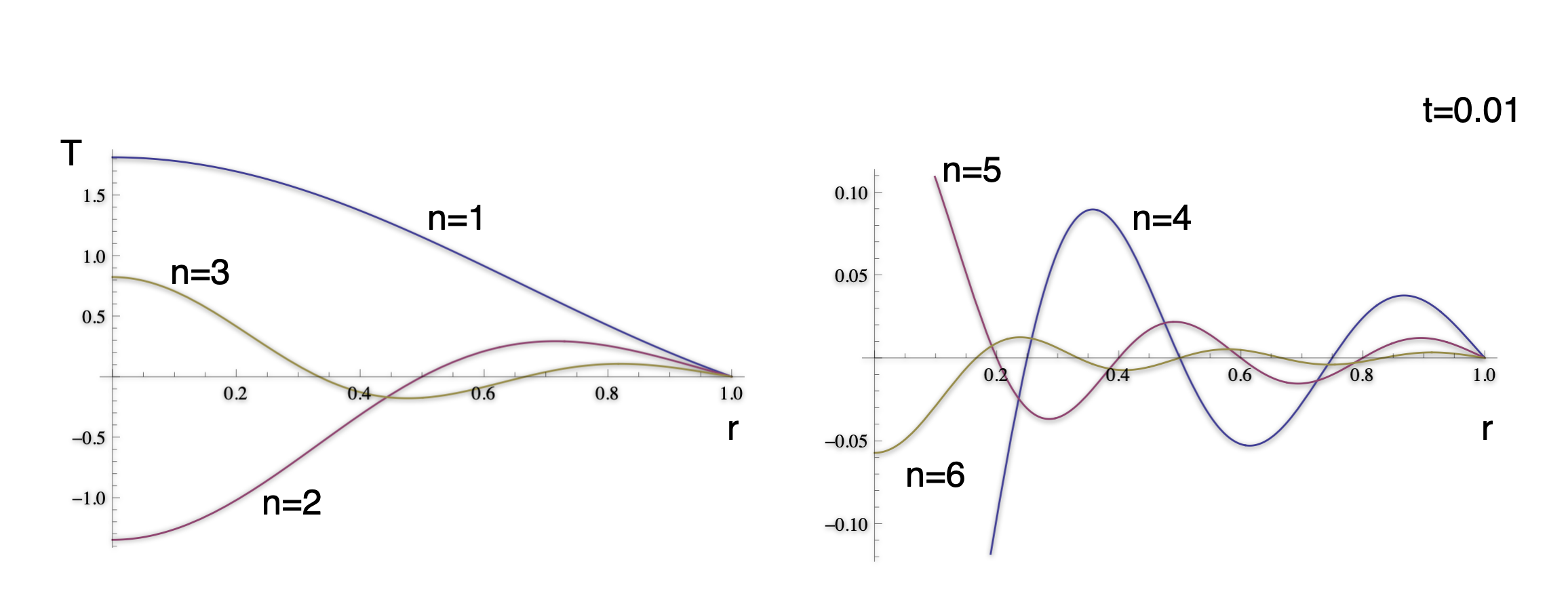
Transient solution for a sphere cooling from a uniform T (details)
\[ T(r,t) = \frac{2}{r} \sum_{n=1}^{\infty} \exp\left( n^2\pi^2 t \right) \sin(n\pi r) \cdot \left( \frac{\sin(n\pi) - n \pi \cos(n\pi)}{n^2 \pi^2} \right) \]
How do the harmonics look when added together to give an approximation to the solution ?
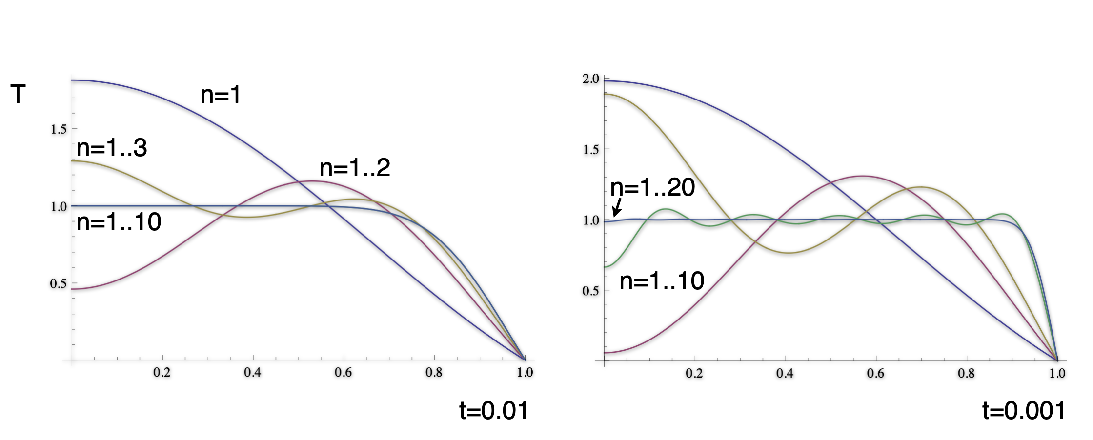
The solution does satisfy the boundary conditions and the physical constraints. Note that the smaller time solution has much sharper gradients and many more terms are required to accurately approximate the solution.
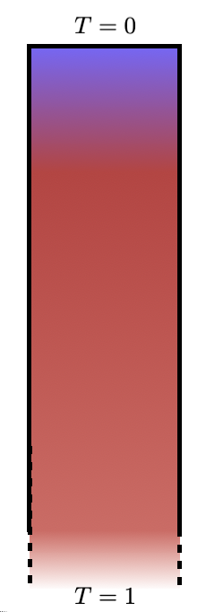
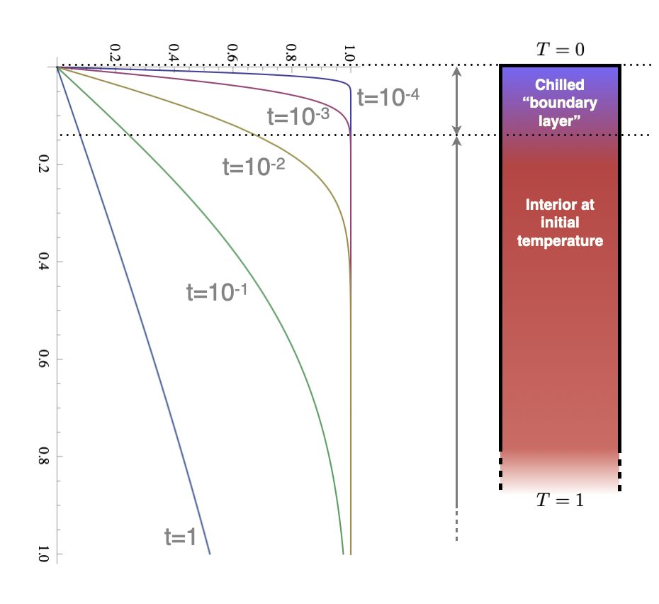
The cooling of a semi-infinite domain
\[ \newcommand{\erfc}{\mathop{\rm erfc}\nolimits} T = \erfc\left(\frac{z}{2\sqrt{t}}\right) \]
This is a very different solution strategy to the cooling sphere (and yet they should, in a mathematical sense, approach each other as the radius becomes large).
The solution looks very similar in character: a cooling front which propagates in from the surface. The curves are self-similar, they just differ by a scaling factor.
The cooling of a semi-infinite domain
This is a problem not unlike the cooling sphere, but with no inherent length scale that comes from the boundary conditions. The equations are similar but we are working in a Cartesian geometry (and also ignoring all the constants !)
\[ \frac{\partial T}{\partial t} = \frac{\partial^2 T}{\partial z^2} \]
This equation simplifies to an ODE if we make the following substitution,
\[ T^* = 1-T; \quad \eta = \frac{z}{2\sqrt{t}} \quad \rightarrow -\eta\frac{d T^*}{d \eta} = \frac{1}{2}\frac{d^2 T^*}{d \eta^2} \]
Which has the following solution
\[ \newcommand{\erf}{\mathop{\rm erf}\nolimits} \newcommand{\erfc}{\mathop{\rm erfc}\nolimits} T^* = 1-\frac{2}{\sqrt{\pi}} \int_0^\eta e^{-\xi^2} d\xi = 1 - \erf(\eta) = \erfc\left(\frac{z}{2\sqrt{t}}\right) \]