EMSC Week 11 - A detailed look at the depth-age relationship for the seafloor.#
We can now try to do what we set out to do - obtain values on an appropriate grid and see what the data look like.
First a grid at fine resolution#
import stripy
import numpy as np

even_mesh = stripy.spherical_meshes.icosahedral_mesh(include_face_points=True, tree=True, refinement_levels=6)
number_of_mesh_points = even_mesh.npoints

latitudes_in_radians = even_mesh.lats
latitudes_in_degrees = np.degrees(latitudes_in_radians)

longitudes_in_radians = even_mesh.lons
longitudes_in_degrees = np.degrees(longitudes_in_radians)%360.0 - 180.0
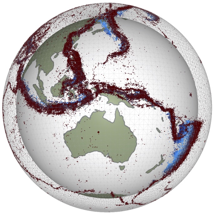
Have a look#
Here we plot the points on the globe to demonstrate that the points are evenly spaced and sufficiently well resolved
import matplotlib.pyplot as plt
%matplotlib inline

import cartopy.crs as ccrs
import cartopy.feature as cfeature

coastline = cfeature.NaturalEarthFeature('physical', 'coastline', '10m',
                           edgecolor=(1.0,0.8,0.0),
                           facecolor="none")

plt.figure(figsize=(7, 7))
ax = plt.subplot(111, projection=ccrs.Orthographic(central_longitude=0.1))

ax.add_feature(coastline, edgecolor="black", linewidth=0.5, zorder=3)

plt.scatter(longitudes_in_degrees, latitudes_in_degrees, s=0.5,
            transform=ccrs.PlateCarree())
Find the age and depth values on these points#
Now we interpolate each of our datasets to the same set of grid points. First we need to define the interpolation routine again.
def map_raster_to_mesh(mesh, latlongrid):

    raster = latlongrid.T

    latitudes_in_radians  = mesh.lats
    longitudes_in_radians = mesh.lons
    latitudes_in_degrees  = np.degrees(latitudes_in_radians)
    longitudes_in_degrees = np.degrees(longitudes_in_radians)%360.0 - 180.0

    dlons = np.mod(longitudes_in_degrees+180.0, 360.0)
    dlats = np.mod(latitudes_in_degrees+90, 180.0)

    ilons = raster.shape[0] * dlons / 360.0
    ilats = raster.shape[1] * dlats / 180.0

    icoords = np.array((ilons, ilats))

    from scipy import ndimage

    mvals = ndimage.map_coordinates(raster, icoords , order=3, mode='nearest').astype(float)

    return mvals
Interpolate age data to fine, triangular grid.#
(You can plot the results as before to see that you have not made a mistake)
plt.figure(figsize=(6, 6))
ax = plt.subplot(111, projection=ccrs.Orthographic(central_longitude=0.1))

ax.add_feature(coastline, edgecolor="black", linewidth=0.5, zorder=3)

plt.scatter(longitudes_in_degrees, latitudes_in_degrees, c=meshages, cmap="RdYlBu",
            vmin=0, vmax=250, s=5,
            transform=ccrs.Geodetic())
import xarray

age_dataset = "data/age.3.6.nc"
age_data = xarray.open_dataset(age_dataset)
subs_data = age_data.sel(x=slice(-180,180, 1), y=slice(-90, 90, 1))

lons = subs_data.coords.get('x')
lats = subs_data.coords.get('y')
vals = subs_data['z']

x,y = np.meshgrid(lons.data, lats.data)
age = vals.data / 100.0
age[np.isnan(age)] = -1.0

meshages = map_raster_to_mesh(even_mesh, age)
Interpolate height data to fine, triangular grid.#
(You can plot the results as before to see that you have not made a mistake)
You also should make a decision about the resolution of the data you want to download.
plt.figure(figsize=(6, 6))
ax = plt.subplot(111, projection=ccrs.Orthographic(central_longitude=0.1))

ax.add_feature(coastline, edgecolor="black", linewidth=0.5, zorder=3)

plt.scatter(longitudes_in_degrees, latitudes_in_degrees, c=meshheights, cmap="terrain",
            vmin=-5000, vmax=5000, s=2,
            transform=ccrs.Geodetic())
(left, bottom, right, top) = (-180, -90, 180, 90)
map_extent = ( left, right, bottom, top)

etopo_dataset = "http://thredds.socib.es/thredds/dodsC/ancillary_data/bathymetry/ETOPO1_Bed_g_gmt4.nc"
etopo_data = xarray.open_dataset(etopo_dataset, engine="pydap")
subs_data = etopo_data.sel(x=slice(left,right, 180), y=slice(bottom, top, 180))

lons = subs_data.coords.get('x')
lats = subs_data.coords.get('y')
vals = subs_data['z']

x,y = np.meshgrid(lons.data, lats.data)
height = vals.data

meshheights = map_raster_to_mesh(even_mesh, height)
plt.figure(figsize=(6, 6))
ax = plt.subplot(111)
ax.set_xlim(0,150)
ax.set_ylim(-7000,-2000)

plt.scatter( meshages[meshheights<-2000], meshheights[meshheights<-2000])
plt.savefig("MyAwesomePlot.png", dpi=250)
Oh No !!#
That looks terrible doesn’t it ? But all is not lost …
Exercise#
Try this: make the points smaller and make them a bit see-through and now take a look. Increase the resolution of your samples in topography. That might make a difference too. Finally, how about trying more grid points ?
Hint: look up the arguments for plt.scatter and see how to use s and alpha.
help(plt.scatter)