PHYS 3070 - S2, 2024
Mantle Dynamics and the Lithosphere
In which we extend our analysis of the surface thermal boundary layer and predict the seafloor depth, and in which we examine the residual signals which might tell us about the mantle
Oceans v. Continents v. Boundary Layers
The ocean basins have a systematic variation in heat flow and thickness from mid ocean ridge to trench that we can interpret in terms of the cooling boundary layer model. The continents do not fit that model at all because they are not part of the global 3D circulation.
Recap from previous lectures
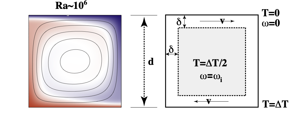
We assume the geometry of fully developed convection is as follows - Thin horizontal boundary layers where heat diffuses into the layer and is carried away by horizontal advection. - These are connected by vertical boundary layers of similar dimension. - Approximately isothermal core, passively rotating, driven by the boundary layers.
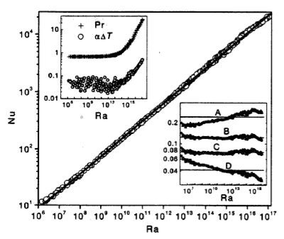
Making all of these assumptions allows us to derive the relationships:
\[ \mathrm{Nu} \propto \mathrm{Ra}^{1/3} \quad \quad \textrm{and} \quad \quad \mathrm{V}_\mathrm{mean} \propto \mathrm{Ra}^{2/3} \]
Recap from previous lectures (2)
We saw that the we could predict the global heat flow by understanding the basic fluid dynamics of the convecting mantle. How can we verify if our theoretical picture has anything to do with the real Earth ?
We might try to look at the global heat flow to see if the numbers match, but, if we want to identify the convection patterns as well, we might need to look at variations in the heat flow.(e.g. can we see cold and hot regions ?). The problem is …
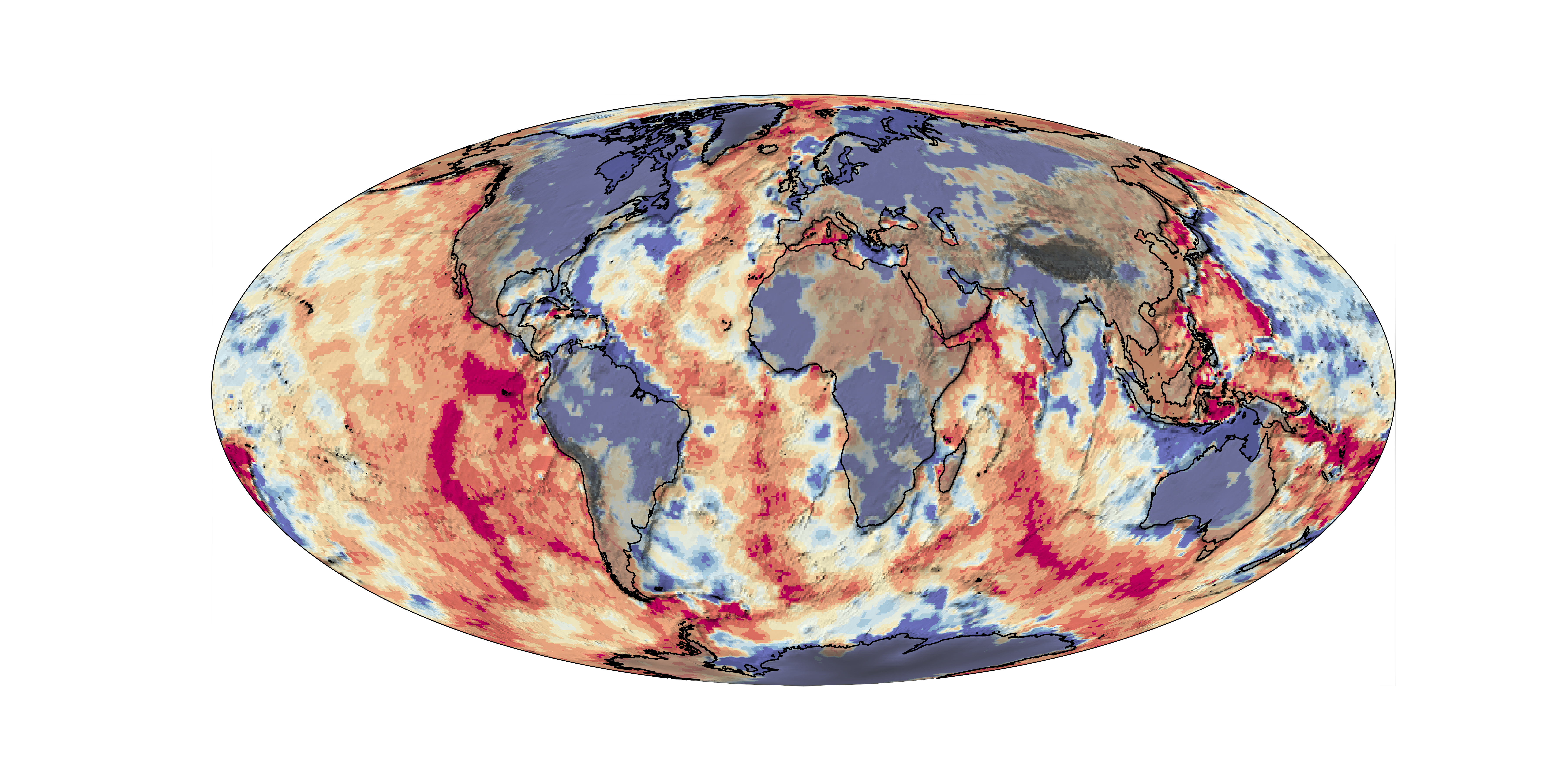
Global Heat Flow
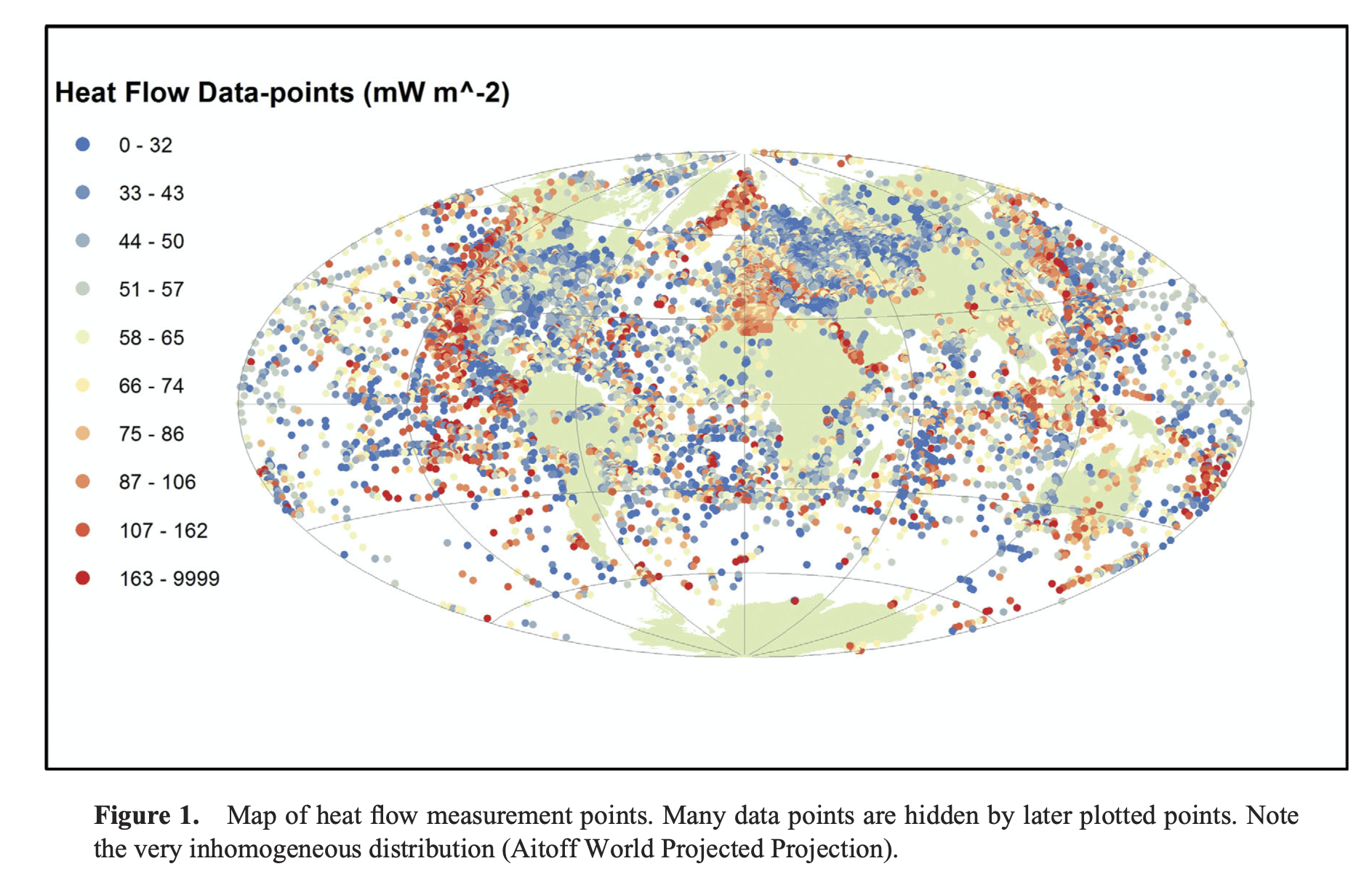
Raw data compiled by Davies & Davies 2013. There are really not very many reliable measurements and the global picture is padded with theoretical values - the ones we would like to test using observations.
Boundary Layer Theory Revisited
We can look a little bit harder at the convective-boundary-layer model we have been using and try to take it one step further.
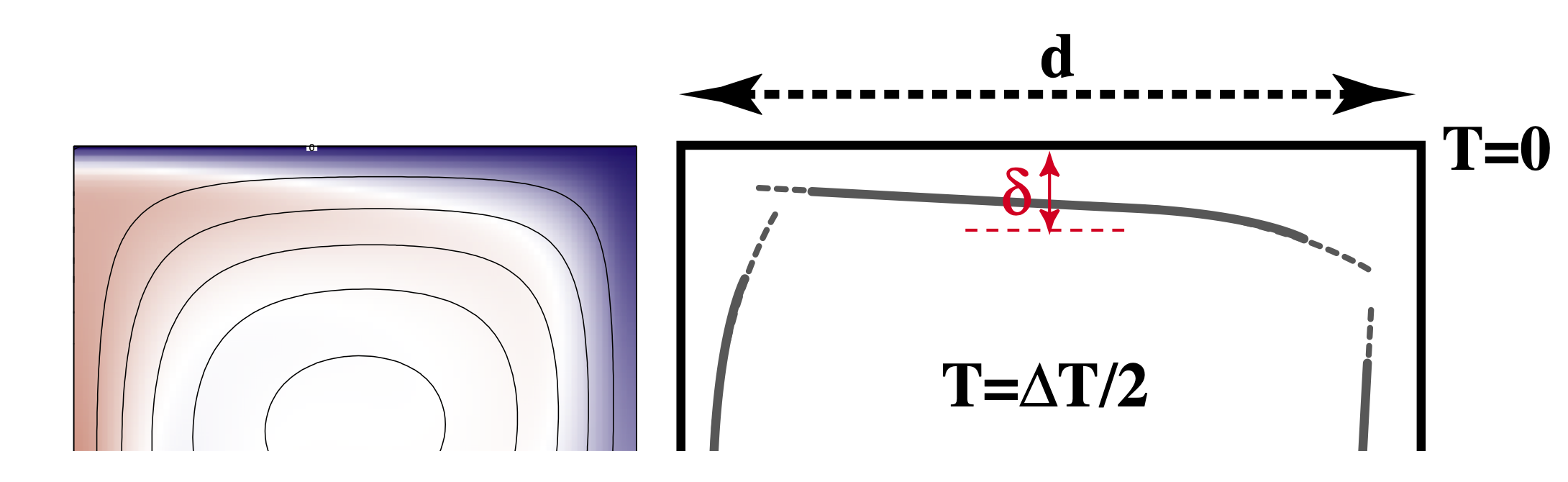
Consider what actually happens as the hot material arrives at the surface (on the left) and spreads out horizontally (to the right). It begins to cool off as it moves. Because the horizontal length scale of the boundary layer is larger than the vertical scale, this is almost like a 1d problem.
Boundary Layer Theory and the Cooling 1/2 Space
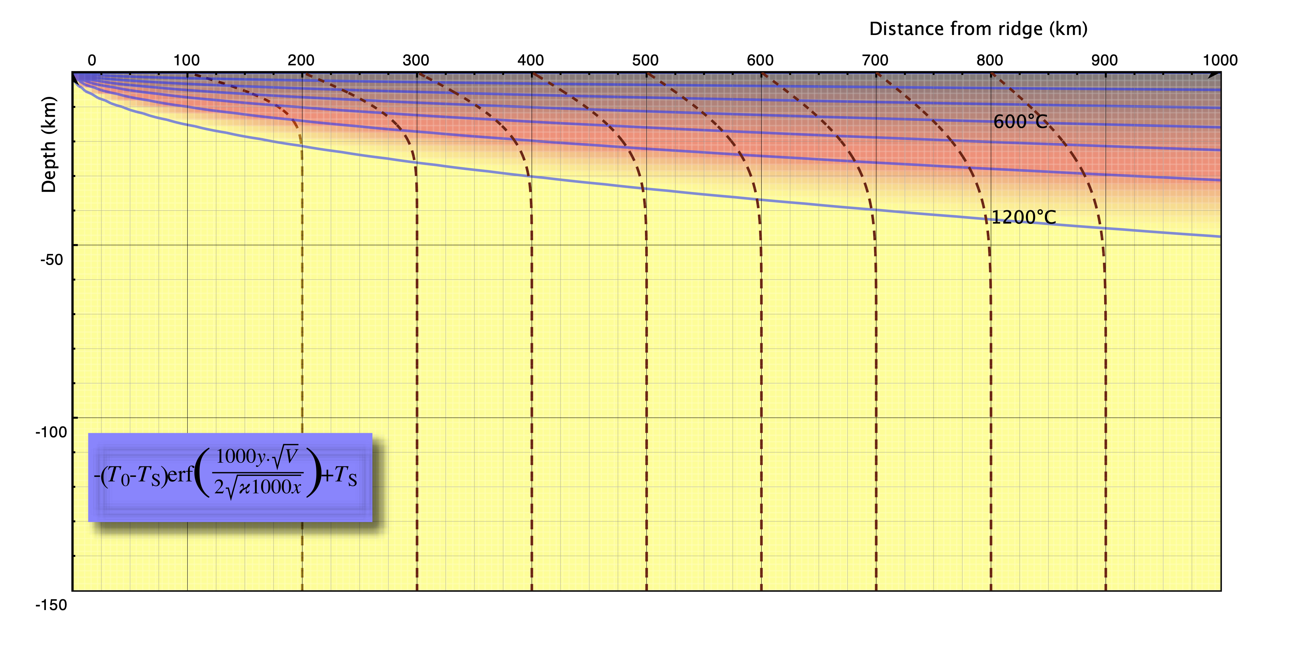
Time and space are not independent in a moving-plate model. If you know the age of the plate and the plate velocity, you also know how far from the ridge you are.
So we can imagine standing on the plate and measuring the geotherm. From this perspective, the plate looks flat and the geotherm is the same all around us. We can model using the cooling half-space solution that we derived in earlier lectures.
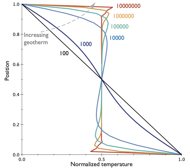
Cooling Lithosphere Thermal Structure
Lithosphere / boundary layer thickness — pick an isotherm and follow it from ridge to trench. Thickness \(\delta\) changes systematically:
\[ \delta \propto \sqrt{\kappa t} \quad \quad \textrm{a.k.a} \quad \quad \delta \propto \sqrt{\kappa x / V} \]
Observations - Ocean Lithosphere Thickness

This predicts the thickness of the thermal boundary layer which can be measured by seismology. NB: the thermal boundary layer is a fuzzy thing without a sharp boundary - seismic methods are not always good at determining this kind of structure.
Observations - Ocean Lithosphere Thickness (2)
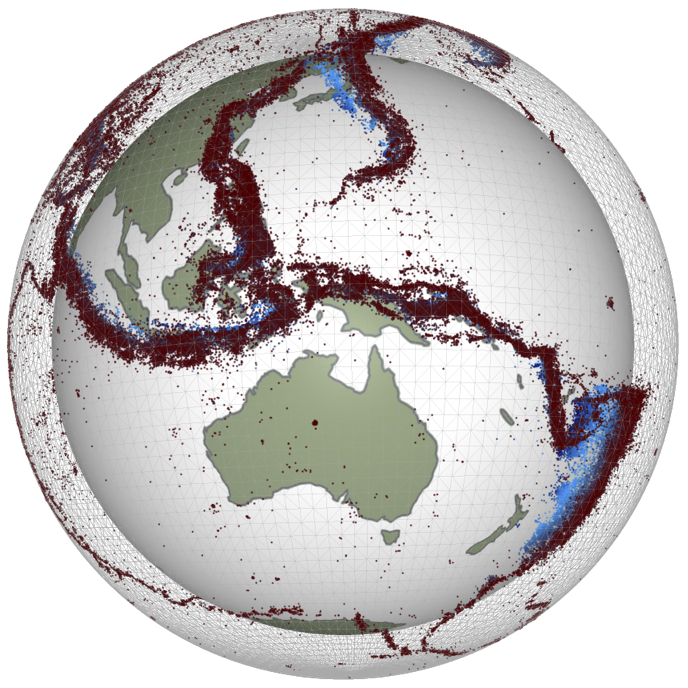
Modern data from the Litho 1.0 global lithosphere model. We can see that there is a signal in the oceans but still this model only sees at a resolution of 1 degree (about 100km).
Colour scale 5km (red); >200km (blue)
Observations - Oceanic Heat Flow
We can differentiate the cooling half-space model to give the temperature gradient at the surface, and hence the heat flux.
The oceanic heat flux is hard to measure at very young ages, but heat flux agrees quite well (at least until about 80-100 Myr)
That is still not a very large number of data points !
Is there a way to turn our boundary layer prediction into a measurement that we can make easily / everywhere ?
Hint: YES (but it may take a little work)

Observations - Oceanic Heat Flow
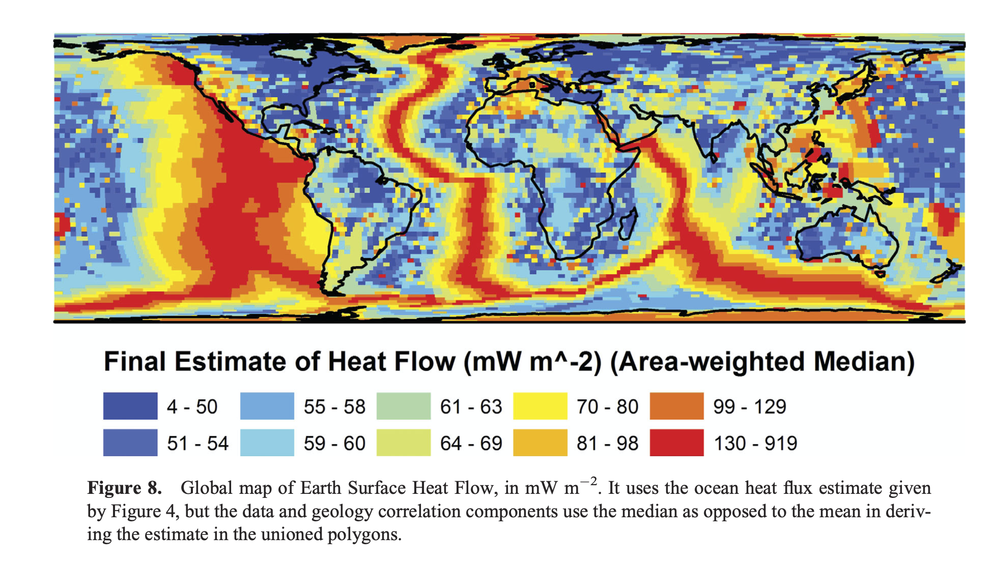
Global heat flow estimate by Davies & Davies 2013 which includes various geological assumptions for different types of heat flow province. **These are not raw / independent data because they use models to interpolate where data are scarce.
Predictions of the Cooling model (80 Myr)
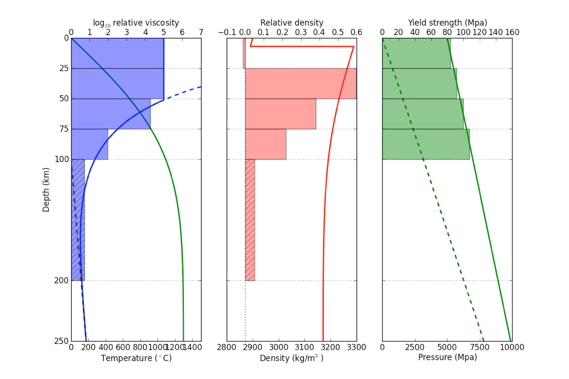
The strength, density plot oceanic lithosphere at 80Myr
Predictions of the Cooling model (120 Myr)
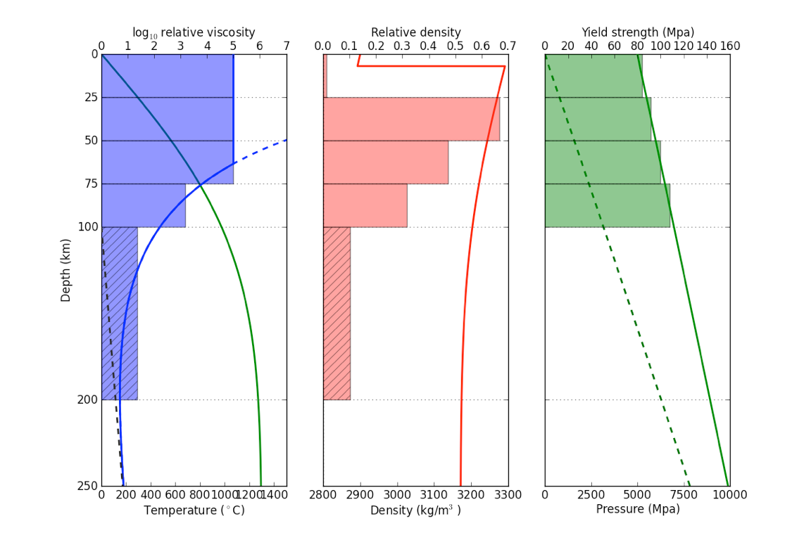
The strength, density plot oceanic lithosphere at 120Myr. (Thicker, denser, stronger)
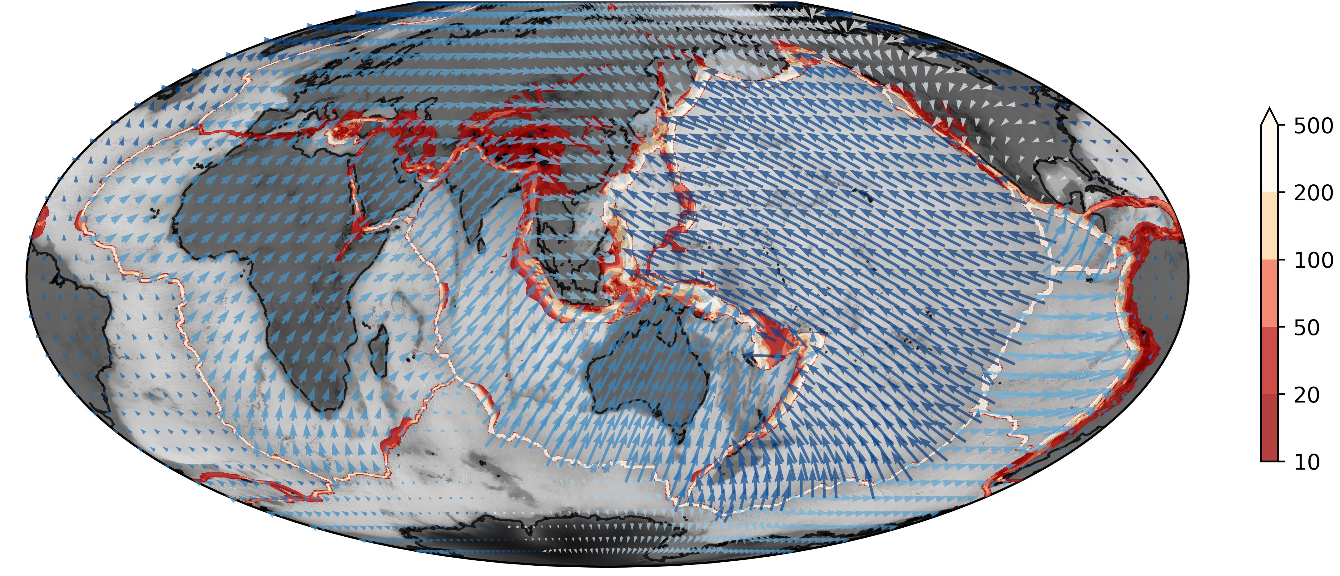
Global Gravity Anomalies
Can we see these density anomalies in the Earth’s gravity field ?

WGM2012 — Bonvalot, S., Balmino, G., Briais, A., M. Kuhn, Peyrefitte, A., Vales N., Biancale, R., Gabalda, G., Reinquin, F., Sarrailh, M., 2012. World Gravity Map. Commission for the Geological Map of the World. Eds. BGI-CGMW-CNES-IRD, Paris
Isostasy and Topography (/ Bathymetry)
We have trouble identifying mass variations for the Earth because of Isostasy which is the phenomenon in which topography and density are causally correlated.
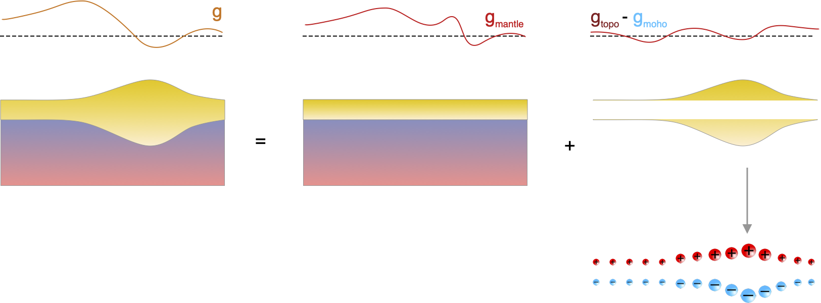
The lack of gravity (anomaly) signature associated with continental topography on Earth is explained simply by ISOSTASY — wherever there is a topographic high, there is a corresponding crustal root which produces a gravitational dipole.
Isostasy and Ocean Depth
If the density varies in a predictable way, then we should be able to see this in an isostatic change in the topography.
\[ \int_0^{d_c} \rho(z) dz = \textrm{constant} \]
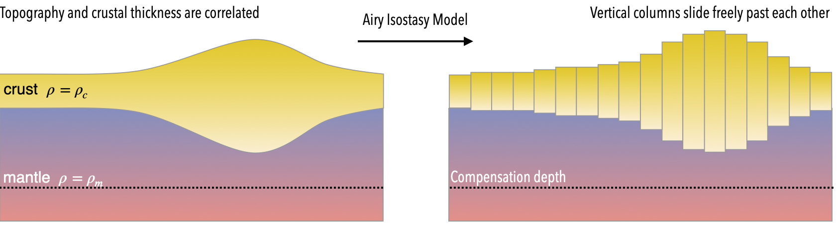
Although we usually think about isostasy as the light crust floating on the mantle, the same approach works for any density variations near the surface (e.g. thermal anomalies). If we integrate every density anomaly in adjacent columns, they balance out in the asthenosphere. This is the Pratt model of isostasy.
Isostasy and Seafloor Cooling
Isostasy means that density variations are visible in the Earth’s topography. This is a good thing for us because topography (bathymetry) is much easier to measure than the other observables.
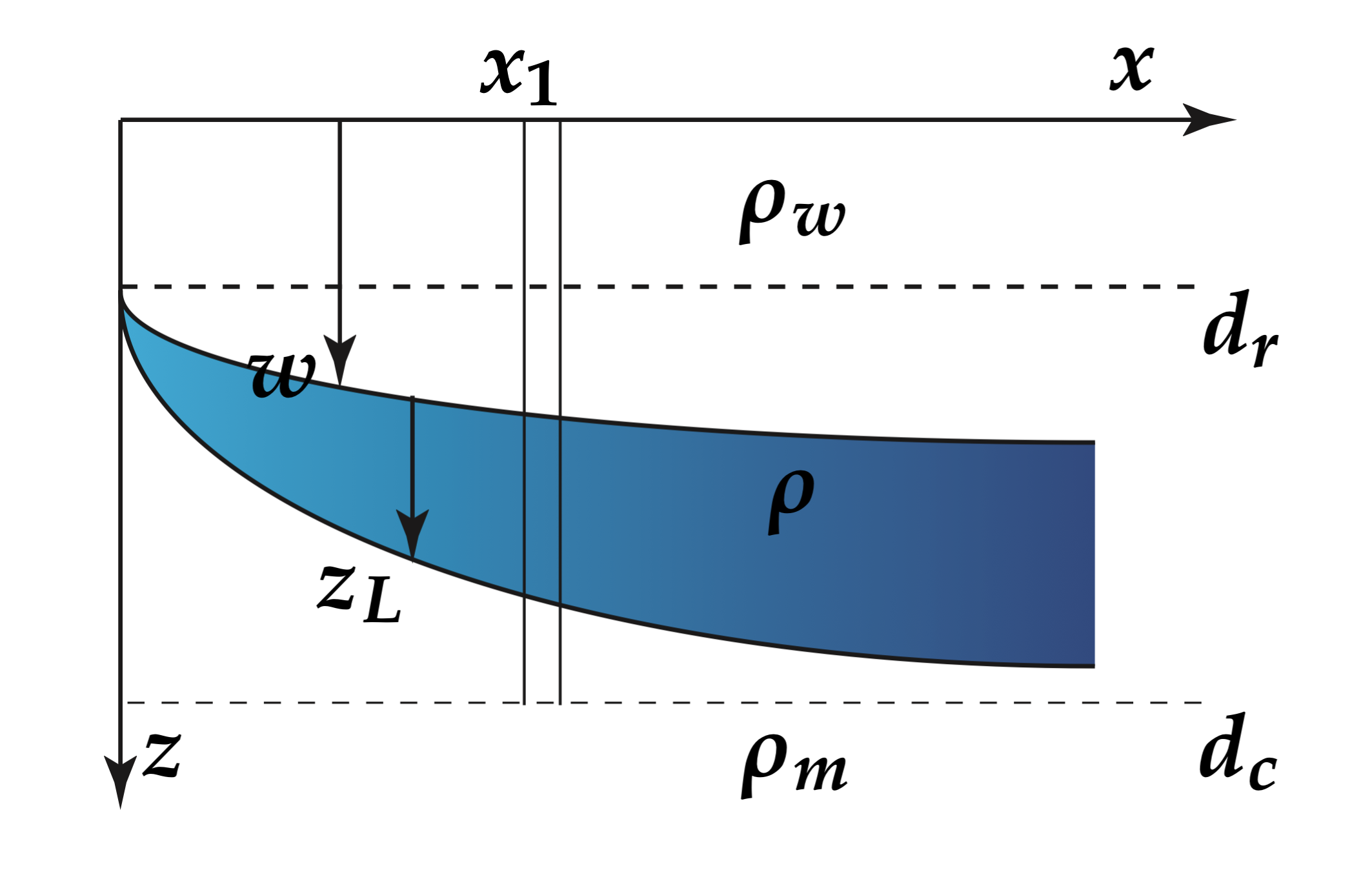
\[\int_{d_r}^{d_c} \rho(z) dz = \rho_m (d_c - d_r)\]
Assume no density variations in the water column or beneath the boundary layer and compare the density column at any given  with the column at 
\[ w \rho_w + \int_{w}^{z_L} \rho(z) dz = \rho_m z_L \]
Isostasy and Sea Floor Age / Depth

Suppose we know how to integrate the Half-Space Cooling equations, then we can compute the water depth as a function of lithospheric age and make a testable prediction:
\[ w = \frac{2 \rho_m \alpha \left(T_1 - T_0\right) }{ \rho_m-\rho_w} \left(\frac{\kappa t}{\pi }\right)^{1/2} \]